Microfacet Theory - Physically Based Rendering

Roughness Using Microfacet Theory - PBRT

引入

物体在宏观上有一个法线$n$，而由于真实的表面都是坑洼不平的，对于微观的一束光，其会命中表面的一个倾斜的片（微表面）而反射出去，这个倾斜面片的法线往往和宏观的$n$方向不同。对于同一个表面从大量的光的统计上来看，越粗糙偏离的也就越大。

当然，如果我们有一个非常强悍的机器，我们可以做一个分辨率很高的模型，其表面具有真正坑坑洼洼的三角形，但是这样做时间、空间的效率都很差。

有意思的是，大量的微表面可以在统计学意义上被建模，从而让基于微表面理论的BSDF不用再受制于上面提到的问题。

光学模型

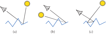
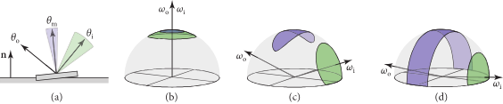
图片展示了三种光学行为
(a): 遮挡，相机看不到被照亮的地方，被其他的微平面挡住了
(b): 阴影，相机看到的地方没有光的照射，因为光线被其他的微平面挡住了
(c): 来回反射(Interreflection), 光线在微表面之间反射，最终能被相机看到

广泛使用的微表面 BSDFs 忽略来回反射。其主要由两个部分组成，一是微表面朝向的统计分布，二是描述光线如何从单个微表面散射的 BSDF

假设光源和观察者相对于微表面的尺度而言足够远的前提下，精确的表面轮廓（那些微表面的具体形状）对于遮蔽和阴影的影响相对较小。

数学推导

微表面分布项 $D(\omega_m)$

我们先不考虑遮挡和阴影，我们首先讨论法线和粗糙度的关系，而我们需要知道有多少比例的微观法线指向了某个特定方向。

我们定义$D(\omega_m)$给出的是法线朝向为 $\omega_m$ 的微表面 (microfacets) 的相对微分面积，给 $D$ 一个方向（$\omega_m$），它会告诉你“有多少(宏观面积一个 $dA$中的)微观法线正指向这个方向”

所有到达 $dA$ 这个小区域的入射光线（$\omega_i$）都是互相平行的。
所有离开 $dA$ 这个小区域的出射光线（$\omega_o$）也都是互相平行的

其有如下关系：
$\int_{H^2(\bold{n})} D(\omega_m) (\omega_m \cdot \bold{n}) d\omega_m = \int_{H^2(\bold{n})} D(\omega_m) \cos \theta_m d\omega_m = 1$
表示一块粗糙的表面，无论它内部多么凹凸不平，它在宏观世界（比如被太阳光照射）的总‘占地面积’是不会变的。

注意，这里的 $\bold{n}$ 在标准反射坐标系（standard reflection coordinate system）下，有 $\bold{n} = (0,0,1)$， 那么 $\omega_m \cdot \bold{n}$ 等价于 $\cos \theta_m$

$\int_{H^2(\bold{n})} D(\omega_m) \cos \theta_m d\omega_m = 1$

• $\int_{H^2(\bold{n})} \dots d\omega_m$ 检查所有（$\int$）可能的倾斜方向（$d\omega_m$）
• $D(\omega_m)$ 朝向 $\omega_m$ 这个方向的微表面占比是多少
• $\theta_m$ 是微表面的法线 $\omega_m$ 和“底座”法线 $\bold{n}$（垂直向上）的夹角 $\cos \theta_m$ 描述了其（投影在宏观上的）投影的面积
• $D(\omega_m) \times \cos \theta_m$ 表示所有朝向 $\omega_m$ 的木片，它们在平坦底座上的‘投影’总面积
• $\int \dots = 1$ 表示所有投影面积的总和，必须等于 1

最常见的微表面分布类型是各向同性的 (isotropic)，这也会导出一个各向同性的聚合 BSDF。
回想一下，当表面绕着宏观表面法线旋转时，一个各向同性的 BSDF 其局部的散射特性是不会改变的

在各向同性的情况下，使用球坐标参数 $\omega_m = (\theta_m, \phi_m)$ 会得到一个只依赖于仰角 $\theta_m$ 的分布。

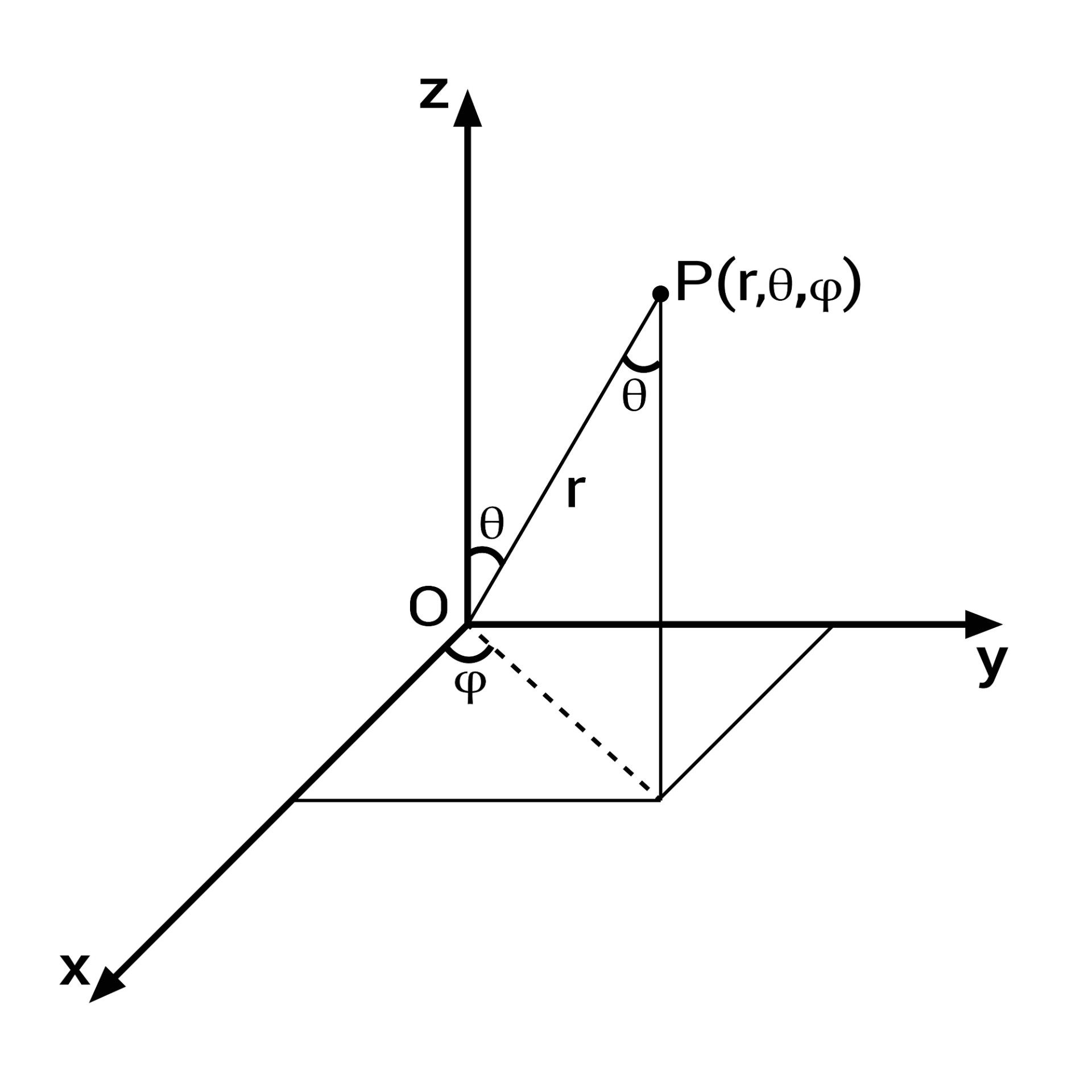
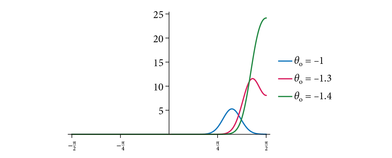
X 轴 ($\theta_m$)： 微观法线的倾斜角度
Y 轴 ($D(\omega_m)$)： 法线的数量（密度）

“长尾”（来自 $\theta_m$ 很大的法线）会捕捉到光，并将其散射开，形成一个非常宽广、非常柔和的“朦胧光晕”

具体实现

那么我们怎么具体去实现D的分布呢？不同的论文有不同的实现，目前比较主流的是GGX与 Disney 实现。
注意，在 D F G 三项中，一般F是通用的，而D与G项配对使用

GGX中的$D(\omega_m)$

$D(\omega_m) = \frac{1}{\pi \alpha_x \alpha_y \cos^4 \theta_m \left( 1 + \tan^2 \theta_m \left( \frac{\cos^2 \phi_m}{\alpha_x^2} + \frac{\sin^2 \phi_m}{\alpha_y^2} \right) \right)^2}$
其中，

• $\omega_m$ 是微观法线方向
• $\theta_m$ 是微观法线 $\omega_m$ 与宏观法线 $\bold{n}$ 之间的仰角
• $\phi_m$ 是微观法线 $\omega_m$ 绕着宏观法线 $\bold{n}$ 旋转的方位角
• $\alpha_x$ 和 $\alpha_y$ 是分别控制两个切线方向（x 和 y）的粗糙度参数
  可以看出，$\alpha_x$ 和 $\alpha_y$ 这两个是属于材质的参数。

三种情况

1. $\alpha_u = \alpha_v = 0$ (完美光滑)

   • $1/\alpha_u$ 和 $1/\alpha_v$ 都是无限大。
   • 这意味着那个椭球体在 U 和 V 两个方向上被无限拉伸。
   • 一个被无限拉伸的球体是什么？就是一个无限平坦的平面。
   • 结果： 完美镜面反射。

2. $\alpha_u = \alpha_v$ (各向同性 / Isotropic)

   • U 方向的粗糙度和 V 方向的粗糙度相等。
   • 微观椭球体被均匀拉伸，变成了球形或“煎饼”形。
   • 结果： 这是一个均匀粗糙的表面，比如磨砂塑料。你绕着法线旋转它，高光不会变。这就是“方位角依赖性消失了”的意思。

3. $\alpha_u \neq \alpha_v$ (各向异性 / Anisotropic)

   • U 方向的粗糙度和 V 方向的粗糙度不相等。
   • 例如，$\alpha_u = 0.5$ 但 $\alpha_v = 0.1$。
   • 这意味着椭球体在 U 方向上“比较粗糙”（没怎么拉伸），但在 V 方向上“比较光滑”（被拉伸得很多）。
   • 结果： 这就是“雪茄”形，它在微观上形成了“凹槽”。这就是有方向的粗糙，比如拉丝金属或木纹

特性

GGX 模型正确地指出：即使在粗糙的表面上，也存在着大量非常倾斜（$\theta_m$ 很大）的微观法线

核心的高光（来自 $\theta_m$ 较小的法线）依然明亮且集中

“长尾”（来自 $\theta_m$ 很大的法线）捕捉到的光，会向四周散射，形成一个非常宽广、非常柔和的“朦胧光晕”

遮蔽项 The Masking Function $G_1(\omega, \omega_m)$

仅有 D 项的话是做不到能量守恒的 BSDF 的。因为从一个特定角度看的时候，不是所有的法线面向这个角度的微平面的面积都会被看到，我们必须避免非物理的能量引入。

我们定义 $G_1(\omega, \omega_m)$，它是一个可见度百分比（一个 0 到 1 之间的折扣因子）
对于所有朝向 $\omega_m$ 的微观法线，当我们从 $\omega$ 方向（可能是观察者方向 $\omega_o$，也可能是光源方向 $\omega_i$）去看它们时，有多少百分比 (fraction) 是没有被挡住的？

$D$ 无法确定 $G_1$ 因为我们无法知道$D$ 给出的法线分布是如何排列的，比如情况 A： 所有的 60° 陡坡都聚集在一起，形成了一面巨大的悬崖。这会投下巨大的阴影。（$G_1$ 会很小）。情况 B： 所有的 60° 陡坡都均匀地、零散地分布在平地中。这只会投下很小的阴影。（$G_1$ 会比较大）

为了便于计算，我们假设是情况B，也就是Smith近似。

$G_1 = 1$ 意味着百分百可见，而$G_1 = 0$意味着0% 可见

从观察者或光源的角度看，表面上的一个微分区域 $dA$ 所呈现的投影面积 (projected area) 为 $dA \cos \theta$，其中 $\theta$ 是该（观察/入射）方向与表面法线 $\bold{n}$ 之间的夹角。

（所有）可见微观表面（图中的粗线）的投影表面积加起来，也必须等于 $dA \cos \theta$。遮蔽函数 $G_1$ 给出的就是 $dA$ 上方总微观表面面积中，在给定方向上可见的比例

数学推导

$\int_{H^2(\bold{n})} D(\omega_m) G_1(\omega, \omega_m) \max(0, \omega \cdot \omega_m) d\omega_m = \omega \cdot \bold{n} = \cos \theta$

• $\int_{H^2(\bold{n})} \dots d\omega_m$ 检查所有（$\int$）可能的倾斜方向（$d\omega_m$）

• $D(\omega_m)$ 朝向 $\omega_m$ 这个方向的微表面占比是多少

• $\omega$ 表示想用来测试这个表面的方向

• $G_1(\omega, \omega_m)$ 在所有法线朝向 $\omega_m$ 的微表面中，当我们从方向 $\omega$（比如相机方向）看过去时，有多少比例 (fraction) 是没有被其他微表面挡住的

• $\max(0, \omega \cdot \omega_m)$ 既负责剔除也负责投影

  • 剔除 (Culling)： $\omega \cdot \omega_m$ 是观察方向 $\omega$ 和微观法线 $\omega_m$ 的点积。如果这个值小于 0（即 $\omega_m$ 背向 $\omega$），$\max(0, \dots)$ 会强制将它变为 0，因为它无论如何都不可见
  • 投影 (Projection)： 如果这个值大于 0（$\omega_m$ 面向 $\omega$），这个点积（即 $\cos \theta_{\omega, \omega_m}$）本身就是一个投影因子。它计算的是这个微观表面 $\omega_m$ 在垂直于 $\omega$ 方向的平面上的“剪影”面积

在上述的公式中，$G_1(\omega, \omega_m)$ 依赖于积分变量$\omega_m$， 而当我们做了 Smith 假设(高度和法线在统计上是独立的)之后，$G_1$ 将不再依赖于它自己的围观法线，其将只依赖于观察方向$\omega$和表面的整体粗糙度。也就是

$$
G_1(\omega, \omega_m) \approx G_1(\omega)
$$

从而，我们得到：

$$
\int_{H^2(\bold{n})} D(\omega_m) G_1(\omega) \max(0, \omega \cdot \omega_m) d\omega_m = \cos \theta
$$

也就是

$$
G_1(\omega) = \frac{\cos \theta}{\int_{H^2(\bold{n})} D(\omega_m) \max(0, \omega \cdot \omega_m) d\omega_m}
$$

虽然上式有解析解，但是为了简便，我们引入坡度域的辅助函数：

$$
G_1(\omega) = \frac{1}{1 + \Lambda(\omega)}
$$

$\Lambda$ 函数（我们之前用它来算 $G_1$）本身就代表了从一个方向看的“不可见”程度

$$
\Lambda(\omega) = \frac{\sqrt{1 + \alpha^2 \tan^2 \theta} - 1}{2}
$$

其中

$$
\alpha = \sqrt{\alpha_x^2 \cos^2 \phi + \alpha_y^2 \sin^2 \phi}
$$

The Masking-Shadowing Function $G$

BSDF 是一个有两个方向参数（$\omega_i$ 和 $\omega_o$）的函数，并且每个方向都受到表面微观结构引起的遮挡效应的影响。
对于观察方向 ($\omega_o$) 和光照方向 ($\omega_i$)，这些（遮挡效应）分别被称为遮蔽 (masking) 和阴影 (shadowing)

为了同时处理这两种情况，（单个方向的）遮蔽函数 $G_1$ 必须被推广为一个遮蔽-阴影函数 (masking-shadowing function) $G_2$，它（$G_2$）给出的是（某个）微分区域中，同时 (simultaneously) 从 $\omega_i$ 和 $\omega_o$ 两个方向都可见的微表面的比例 (fraction)

如果我们假设遮蔽 (masking) 和阴影 (shadowing) 是统计上独立的 (statistically independent) 事件，那么这两个概率就可以简单地相乘：

$$
G_2(\omega_i, \omega_o) = G_1(\omega_i) G_1(\omega_o)
$$

这种假设将会刚高估阴影和遮蔽的实际数量，会导致在最终渲染的图片上出现暗区。因为这两个事件其实在统计学上并不是独立的，而是相关的。一个微表面要么倾向于对“两边”都可见，要么倾向于对“两边”都不可见。 它高估了“一个可见的表面又恰好被另一个挡住”的概率。它错误地把两个 80% 乘在了一起（得到了 64%），而真实的“同时可见”比例（$G_2$）可能要高得多（比如 75%）

为了修复这个问题，我们引入新公式

$$
G_2 = \frac{1}{1 + \Lambda(\omega_i) + \Lambda(\omega_o)}
$$

• 它不再是“概率相乘”（$G_1 \times G_1$）
• 它变成了“不可见量相加”

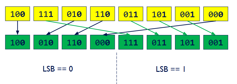
采样

现在我们考虑当一条光线从 $\omega_i$ 方向射入一个粗糙表面时，它接下来应该‘弹’向哪个随机的方向 $\omega_o$

• 光线会“弹”向哪里，取决于它击中了哪一个微观法线 $\omega_m$

• 它不能用一个“公平的”骰子（比如在所有方向上均匀抽样），因为我们知道，击中某些 $\omega_m$（比如那些正对着它的）的概率要高得多

一条光线与某个特定微表面相互作用的概率，是与它的可见面积 (visible area) 成正比的。换句话说，一束光（或视线）击中某个微表面的概率，正比于那个微表面向它呈现的可见投影面积

原公式（确保所有“可见”微表面投影的总面积是 $\cos \theta$ * $dA$）

$$
\int_{H^2(\bold{n})} D(\omega_m) G_1(\omega) \max(0, \omega \cdot \omega_m) d\omega_m = \cos \theta
$$

这是所有法线朝向 $\omega_m$（附近 $d\omega_m$ 范围内）的可见微表面，它们所贡献的投影面积总和：

$$
D(\omega_m) G_1(\omega) \max(0, \omega \cdot \omega_m) d\omega_m
$$

当一束光（或我们的视线）从方向 $\omega$ 射向这块表面时，它击中一个法线朝向为 $\omega_m$ 的微表面的（法线空间）概率是多少？:

$$
D_\omega(\omega_m) = \frac{G_1(\omega) D(\omega_m) \max(0, \omega \cdot \omega_m)}{\cos \theta} \quad
$$

$$
D_\omega(\omega_m) = \frac{\text{朝向 }\omega_m\text{ 的可见投影面积}}{\text{所有可见投影面积的总和}}
$$

也就是我们给$D$一个向量，其会返回 $\omega_m$ 被击中的概率是 $X$

而Sample() (采样算法)是“骰子”

• 作用这是一个生成函数。
• 输入： 它通常只需要 1 或 2 个 0 到 1 之间的随机数（比如 rand(), rand()）。
• 输出： 它“吐出”一个全新的、随机的向量 $\omega_m$（“这是我帮你‘摇’出来的方向！”）。

那么如果说完全随机地去得到方向，最后调用$D_{\omega}(\omega_m)$来事后告诉我们这个随机 $\omega_m$ 的概率是 $0.0001%$，这个渲染器是可以工作的，但是十分低效。

我们需要重要性采样，我们在得到方向地时候，这个随机方向的产生器就要产生更多的高概率方向，而较少地产生低概率方向。

那么如何制作这样的采样器呢？有数学上的方法，但是有一个相对简单的几何途径可以做到。

几何方法（可见法线采样）

1. 在代码中，假想一个由粗糙度 $\alpha_x, \alpha_y$ 定义的标准GGX椭球体
2. 计算这个“椭球体”从方向 $\omega$ 看过去的2D剪影 (2D silhouette)
3. 在这个2D剪影上，均匀地 (uniformly) 随机选择一个 2D 点 $(u, v)$
4. 从这个 2D 点 $(u, v)$，沿着 $\omega$ 方向“逆向”投射回3D椭球体上，找到那个唯一的撞击点 $p$
5. 获取这个 3D 撞击点 $p$ 在椭球体上的表面法线 $\omega_m$

• 这个方法已经处理了遮蔽

微观“凸起”的 2D 剪影的形状，会根据你的“观察角度 $\omega$”而改变。这个算法必须精确地模拟这个改变

The Torrance–Sparrow Model

1. 给定一个来自方向 $\omega$ 的观察光线，我们使用‘可见法线采样’（“骰子”），从**可见法线分布$D_\omega(\omega_m)$（“裁判”）所定义的概率中，生成 (sample) 一个微观法线 $\omega_m$**。并且，我们同时会使用$D_\omega(\omega_m)$ 这个公式，来计算出我们刚刚生成的那个 $\omega_m$ 所对应的概率密度值（一个数字/Float）

   • 这一步（在概念上）封装了“观察光线”与“随机的微观结构”求交 (intersecting) 的过程
   • 注意，这一步产生的$\omega_m$可能会相对于原宏观$\bold{n}$偏离很大，从而导致从一些角度射进来的光线，会被反射到V型谷的深处，而非去向摄像机，然后也许会经历多次反弹，最终射向摄像机。但是，Smith’s GGX的数学模型没有包括这种情形，导致了能量损失，其较为粗略地将这样的光线终止。当材质非常粗糙的时候，这种情况将会很常见。有一些研究进行了对这种情况的不同程度的修补。如 Fast-MSX: Fast Multiple Scattering ApproximationFast-MSX

2. （光线）在被采样的微表面上的反射，是使用镜面反射定律 (law of specular reflection) 和菲涅尔方程 (Fresnel equations) 来建模的

   • 这会（反向）推导出一个入射方向 $\omega_i$，以及一个反射系数 (reflection coefficient)，该系数会衰减 (attenuates) 这条路径所携带的光

3. 最终，散射的光会（再）乘以一个 $G_1(\omega_i)$，以计入其他微表面所造成的阴影效应

在渲染器中，我们有来自上一次光的交互带来的$\omega_o$，我们要算出$\omega_i$ 以及其对应的概率密度，并完成采样。

想象一个法线 $\omega_m$。向量 $\omega_o$ 和 $\omega_i$ 在 $\omega_m$ 的两侧对称
注意：在 PBRT 的约定中，所有向量 $\omega_i, \omega_o, \omega_m$ 都指向外

根据镜面反射关系，有：
$\omega_i = -\omega_o + 2(\omega_m \cdot \omega_o) \omega_m$

$\omega_m = \frac{\omega_i + \omega_o}{|\omega_i + \omega_o|}$

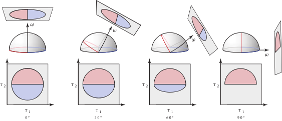
我们固定出射方向 $\omega_o$，并可视化一组微表面（用蓝色阴影表示），这些微表面能将来自入射方向（用绿色阴影表示）周围的一个弧/锥的光线有效反射出去

• 在 (a) 所示的二维平面 (flatland) 设置中，这组有效的微表面 (admissible microfacets) 只是一个更小的弧。3D 情况则更复杂，涉及到球面圆锥截面 (spherical conic sections)。
• 在 (b) 中，当 $\omega_i$ 锥体的中心与 $\omega_o$ 对齐时，有效的微表面形成一个球面圆形 (spherical circle)。
• 在 (c) 中，当 $\omega_o$ 与 $\omega_i$ 锥体中心方向之间呈 $45^{\circ}$ 角时，有效的微表面形成一个球面椭圆 (spherical ellipse)
• 在 (d) 中，当角度为 $90^{\circ}$ 时，结果则是一个球面双曲线 (spherical hyperbola)

我们想要知道最终选出的$\omega_i$的概率密度是多少，而非$\omega_m$,他们的关系是：

$p(\omega_i) d\omega_i = p(\omega_m) d\omega_m$
$p(\omega_i) = p(\omega_m) \times \frac{d\omega_m}{d\omega_i}$

我们先关注 $\frac{d\omega_m}{d\omega_i}$，其表示在 $\omega_m$ 空间中一个无限小的立体角 $d\omega_m$”，除以“在 $\omega_i$ 空间中对应的那个无限小的立体角 $d\omega_i$。

而又有，在球面坐标中，微分立体角 $d\omega = \sin\theta d\theta d\phi$

$$
\frac{d\omega_m}{d\omega_i} = \frac{\sin \theta_m d\theta_m d\phi_m}{\sin \theta_i d\theta_i d\phi_i}
$$

$$
\begin{aligned}
\frac{d\omega_m}{d\omega_i} &= \frac{\sin \theta_m d\theta_m d\phi_m}{\sin (2\theta_m) (2 d\theta_m) (d\phi_m)} \
&= \frac{\sin \theta_m}{ (2 \sin \theta_m \cos \theta_m) \cdot 2} \
&= \frac{1}{4 \cos \theta_m} \
&= \frac{1}{4(\omega_i \cdot \omega_m)} = \frac{1}{4(\omega_o \cdot \omega_m)}
\end{aligned} \quad
$$

也就是

$$
p(\omega_i) = D_\omega(\omega_m) \times \frac{1}{4(\omega_o \cdot \omega_m)}
$$

BSDF

evaluate 公式的推导：

回顾一下渲染方程：
$L_o(\text{p}, \omega_o) = \int_{H^2(\mathbf{n})} f_r(\text{p}, \omega_o, \omega_i) L_i(\text{p}, \omega_i) |\cos \theta_i| d\omega_i$
单样本蒙特卡洛估计器：

$$
\approx \frac{f_r(\text{p}, \omega_o, \omega_i) L_i(\text{p}, \omega_i) |\cos \theta_i|}{p(\omega_i)}
$$

结合在一起，有

$$
\begin{aligned}
L_o(\text{p}, \omega_o) &= \int_{H^2(\mathbf{n})} f_r(\text{p}, \omega_o, \omega_i) L_i(\text{p}, \omega_i) |\cos \theta_i| d\omega_i \
&\approx \frac{f_r(\text{p}, \omega_o, \omega_i) L_i(\text{p}, \omega_i) |\cos \theta_i|}{p(\omega_i)}
\end{aligned}
$$

Torrance–Sparrow 模型给出的单光线的辐射亮度，应该和蒙特卡洛估计相一致：

$$
\frac{f_r(\text{p}, \omega_o, \omega_i) L_i(\text{p}, \omega_i) |\cos \theta_i|}{p(\omega_i)} \stackrel{!}{=} F(\omega_o \cdot \omega_m \text{(反射角度)}) G_1(\omega_i) L_i(\text{p}, \omega_i)
$$

把两边的 $L_i$ 消掉，有

$$
\frac{f_r \cdot |\cos \theta_i|}{p(\omega_i)} = F(\omega_o \cdot \omega_m) G_1(\omega_i)
$$

移项，有

$$
f_r = \frac{F \cdot G_1(\omega_i) \cdot p(\omega_i)}{|\cos \theta_i|}
$$

代入 $p(\omega_i)$，有

$$
p(\omega_i) = p(\omega_m) \times \frac{d\omega_m}{d\omega_i}
$$

而$p(\omega_m)$是：

$$
p(\omega_m) = D_\omega(\omega_m) = \frac{G_1(\omega_o) D(\omega_m) (\omega_o \cdot \omega_m)}{(\mathbf{n} \cdot \omega_o)}
$$

$\frac{d\omega_m}{d\omega_i}$ 是：
$\frac{d\omega_m}{d\omega_i} = \frac{1}{4 (\omega_o \cdot \omega_m)}$
则有：

$$
p(\omega_i) = \frac{G_1(\omega_o) D(\omega_m)}{4 (\mathbf{n} \cdot \omega_o)}
$$

则有：

$$
f_r = \frac{F(\omega_o \cdot \omega_m) \cdot G_1(\omega_i) \cdot p(\omega_i)}{(\mathbf{n} \cdot \omega_i)}
$$

则有：

$$
f_r = \frac{F(\omega_o \cdot \omega_m) \cdot G_1(\omega_i) \cdot \left[ \frac{G_1(\omega_o) D(\omega_m)}{4 (\mathbf{n} \cdot \omega_o)} \right]}{(\mathbf{n} \cdot \omega_i)}
$$

然而，这个 $G = G_1 \times G_1$ 的“非相关”几何项会导致渲染过暗。因此，在最终的实现中，我们将其替换为物理上更精确的“高度相关”模型 $G_2 = \frac{1}{1 + \Lambda(\omega_i) + \Lambda(\omega_o)}$

参考
3-Parallel-Algorithms.pptx

Parallel Reduction

Arithmetic intensity: compute to memory access ratio 进行一次内存访问时，可以执行多少次计算操作。这个比值越大，往往意味着性能更好。

找到数组的和，最大值，连续积，均值

Reduction:  An operation that computes a single result from a set of data

在并行计算中，为了高效地对大量数据进行规约操作（如求和、求最大值等），算法通常采用迭代的形式。在每一轮迭代中，活动的线程会将两两配对的元素进行运算，从而将数据规模减半（因为每次迭代数据都会减半，往往是$\log_2{n}$次迭代）

数组的和

分治分冶，两个两个地求和下去
$O(logn)$ for n elements

第一行的$\log_2{n} -1$ 指的是总共的迭代次数 - 1，第一行的for是用来遍历迭代的，di表示是低几次迭代

第二行的all意味着并行，k是线程的索引， 步长为$2^{d+1}$，与迭代次数有关。例如， 若若当前迭代为第0次，那么步长为$2$，如果是第1次迭代，步长为$4$，如果是第2次迭代，步长为$8$

第三行执行了加法的具体内容。

当第0次迭代时（d=0）

1
2

for all k = 0 to n -1 by 2 in parallel
	x[k + 1] += x[k]

即，
线程0，执行x[0 + 1] += x[0]，也就是 x[1] += x[0]

线程2，执行x[2 + 1] += x[2]，也就是 x[3] += x[2]

线程4，执行x[4 + 1] += x[4]，也就是 x[5] += x[4]

以此类推…

当第1次迭代时（d=1）

1
2

for all k = 0 to n -1 by 4 in parallel
	x[k + 3] += x[k + 1]

即，
线程0，执行x[0 + 3] += x[0 + 1]，也就是 x[3] += x[1]

线程4，执行x[4 + 3] += x[4 + 1]，也就是x[7] += x[5]

Scan

All-Prefix-Sums 前缀和（前缀规约）

这里的⊕指的是二元运算，其需要两个操作数，且满足结合律运算，即(a⊕b)⊕c=a⊕(b⊕c)

$I$ 代表身份元，它是指与任何元素进行二元运算后，结果仍然是该元素的特殊值。

• 对于加法 (+)，身份元是 0，因为 a+0=a
• 对于乘法 (×)，身份元是 1，因为 a×1=a
• 对于最大值 (max)，身份元是 −∞ (负无穷大)，因为 max(a,−∞)=a

结合律对设计并行算法至关重要，因为它允许我们以任何顺序对数据进行分组和处理，而不会影响最终结果。

• Exclusive Scan
  不包括当前指向的数组中的元素
  In: [ 3 1 7 0 4 1 6 3]
  Out: [ 0 3 4 11 11 15 16 22]
• Inclusive Scan(Prescan) 闭扫描
  包括当前指向的数组中的元素
  In: [ 3 1 7 0 4 1 6 3]
  Out: [ 3 4 11 11 15 16 22 25]

如何从一个闭扫描创建开扫描（逆向扫描）？

Input: [ 3 4 11 11 15 16 22 25]
将每一位右移，在首位补Identity（对于这里是0），有
[ 0 3 4 11 11 15 16 22]
Exclusive: [ 0 3 4 11 11 15 16 22]

如何从一个开扫描创建闭扫描（逆向扫描） Prescan？

我们既需要开扫描，也需要原始的输入

$$
Inclusive[i]=Exclusive[i]+Input[i]
$$

将开扫描与原始输入的元素逐个相加，
得到最终结果 [ 3, 4, 11, 11, 15, 16, 22, 25]

A parallel algorithm for Inclusive Scan

对于单线程来说，这个算法很简单。首位照抄原始输入的首位，之后的元素从前一个元素加上原始输入当前的元素即可。

1
2
3

out[0] = in[0]; // assuming n > 0
for (int k = 1; k < n; ++k)
  out[k] = out[k – 1] + in[k];

若如此做，对于n个元素的数组，我们需要执行 n-1 次加法操作。

并行算法的时间复杂度是$O(logn)$，因为其不再必须等待上一步。
一般的并行化算法（Hillis-Steele）可以将工作总量变为$O(nlogn)$ ，而更高效的算法可以将工作总量优化到 $O(n)$

Native Parallel Scan

1
2
3
4
5

for d = 0 to (log₂n) - 1
	for all k in parallel
		if(k >= 2^(d)){
			x[k] = x[k - 2^d] + x[k];
		}

这里的d是指当前处理的是第几次迭代
注意，这里的k步长总是1， 但是其会经过$k >= 2^{d}$ 这个判断来去除一些不需要进行的运算。

由于我们无法控制线程的先后执行顺序，且算法中会出现依靠数组中其他值的情况，例如计算 Array[1] = Array[1] + Array[0]，数组中的元素可能因为被其他值更改而污染。所以在实现中使用乒乓缓存。即，在一个迭代中，只从一个数组中读，只写入另一个数组，然后交换这两个数组。

Work-Efficient Parallel Scan

若如此做，将会首先得到一个开扫描，最后进行一次逆向扫描，得到闭扫描

二叉树

利用一棵平衡二叉树来分两阶段执行Scan

假设输入是[0 1 2 3 4 5 6 7]

• Up-Sweep

1
2
3
4
5

// Same code as our Parallel Reduction
// 注意，这里的to是一个闭区间，包含log_2{n} - 1
for d = 0 to log_2{n} - 1
  for all k = 0 to n – 1 by 2^(d+1) in parallel
    x[k + 2^(d+1) – 1] += x[k + 2^(d) – 1];

% 是取模运算，a % b 的结果是 a 除以 b 后的余数。 6 % 2 = 0

需要指出的是，由于步长的存在，这里伪代码的k是一个稀疏的、跳跃式增长的变量，用来标记每个计算单元的起始位置，是从“外部调度者”的视角来看待的。而CUDA中的k，或者线程id是每个线程自己的视角，那么经过了((k + 1) % fullStride != 0) 这样的判断之后，线程id已经成为了实际写入数据的位置。

也就是说，在kernel函数中，对于每个线程而言，

1
2
3
4
5
6
7
8
9
10
11
12
13

__global__ void kernParallelScan(int paddedN, int n, int d, int* idata) {
    int k = blockIdx.x * blockDim.x + threadIdx.x;

	int halfStride = 1 << (d);
    int fullStride = halfStride * 2;

    if (k >= n || ((k + 1) % fullStride != 0)) {
        return;
    }

    // up-sweep
    idata[k] += idata[k - halfStride];
}

1. Imagine array as a tree
   Array stores only left child
   Right child is the element itself
2. For node at index n
   Left child index = n/2 (rounds down)
   Right child index = n
   

我们把这个树扫（推）上去，得到了上扫完成后的一个中间状态[0 1 2 6 4 9 6 28]

• Down-Sweep
  “下扫”的核心思想是：从树的根节点开始，将每个节点所代表的“前缀和”分配给它的子节点，直到最底层的叶子节点（也就是我们的目标数组）

1. 树顶的值换成0
2. 从上至下地，一层层地，父节点把自己的值传给左孩子，把“自己的值 + 左孩子的原始值”传给右孩子

在得到我们上扫的结果后：

我们执行下列步骤：

1. 根节点的值被设置为了0（注意，这一步应该只执行一次，而不是并行时，每个线程都这样设置一下，因为对于非第一个执行的线程，其根节点已经被第一个执行的线程更新过了）

2. 蓝色层的6，拷贝父节点的值，新值变为了0；蓝色层的22，拷贝父节点的值，加上左边兄弟的原值6，新值变为6。 也就是蓝色这一层变为了[6, 22]

3. 绿色这一层进行运算。
   绿色1，拷贝父节点的值，新值为0， 绿色5，拷贝父节点的值，加上左兄弟原值，变为1

绿色9，拷贝父节点的值6，新值为6，绿色13，拷贝父节点 6，再加上左边兄弟（绿色9）的原始值 9。新值为 6 + 9 = 15。
它们的值变成了 [0, 1, 6, 15]

5. 黄色这一层进行运算，有新的黄色层[0 0 1 3 6 10 15 21]，即开扫描

6. 将开扫描加上原始输入，有闭扫描

• Up-Sweep
  $O(n)$ adds
• Down-Sweep
  $O(n)$ adds
  $O(n)$ swaps

减少加法操作次数？

Stream Compaction

类似于std::copy_if

在GPU的时候我们就把不要的数据给丢了，这样最终需要从GPU传到CPU的
数据量就少了很多。

Why scan?

• Preserve the order
• meet certain criteria

Step 1: Compute temporary array containing

• 1 if corresponding element meets criteria
• 0 if element does not meet criteria

Step 2 Run exclusive
scan on temporary array

这里第一行是原始数据，绿色表示满足了条件，红色表示未满足条件

黄色是临时数组

蓝色是临时数组的开扫描

Step 3 Scatter

• Results of scan is index into final array
• Only write an element if temporary array has a 1

那么利用这个开扫描，我们可以知道要开一个多大的数组，也就是最后一位值，且知道每一个要写的元素将会写的index

Summed Area Table （SAT）

2D table where each element stores the sum of all elements in an input image between the lower left corner and the entry location.

SAT的本质是一个二维的包含式前缀和。

通过一次预计算，使得我们可以在“固定的时间”内，极速计算出图像中任意矩形区域内所有像素值的总和（以及平均值）

它的最大优点是，可以用 固定的时间O(1) 对图像的每个像素应用任意尺寸的矩形滤镜。即计算一个 3x3 小方框内所有像素的平均值，和计算一个 500x500 巨大方框内像素的平均值，花费的时间是完全相同的。

我们不需要遍历矩形内的每一个像素。我们只需要从一个预先计算好的“和区域表（SAT）”中，读取四个角点的值即可。

$$
s_{filter} = \frac{s_ur - s_ul - s_lr + s_ll}{w \times h}
$$

SAT(D) - SAT(B) - SAT(C) + SAT(A)

以近似景深为例
1.对于屏幕上的每一个像素，我们读取它的深度值。
2. 根据深度值和预设的焦距，计算出这个像素应该有多“糊”。这个模糊程度可以直接转换成一个矩形模糊窗口的尺寸（比如5x5, 15x15等）
3. 利用SAT，我们只需4次查询，就能立刻得到这个动态尺寸的矩形窗口内的像素平均值。
5. 将这个平均值作为该像素的最终颜色

GPU Implementation Inclusive Scan

1. 原始输入

1
2
3

[ 1, 2, 3 ]
[ 4, 5, 6 ]
[ 7, 8, 9 ]

2. 水平扫描
   我们对图像的每一行，独立地执行一次包含式扫描
   第1行: [1, 1+2, 1+2+3] ➔ [ 1, 3, 6 ]

第2行: [4, 4+5, 4+5+6] ➔ [ 4, 9, 15 ]

第3行: [7, 7+8, 7+8+9] ➔ [ 7, 15, 24 ]

即

1
2
3

[ 1,  3,  6 ]
[ 4,  9, 15 ]
[ 7, 15, 24 ]

3. 垂直扫描
   我们对上一步得到的中间结果的每一列，再次独立地执行一次包含式扫描

第1列: [1, 1+4, 1+4+7] ➔ [ 1, 5, 12 ]

第2列: [3, 3+9, 3+9+15] ➔ [ 3, 12, 27 ]

第3列: [6, 6+15, 6+15+24] ➔ [ 6, 21, 45 ]

1
2
3
4

// 最终的 SAT
[  1,  3,  6 ]
[  5, 12, 21 ]
[ 12, 27, 45 ]

Radix Sort

k-bit keys require k passes k比特的键需要k轮处理

如果要对一个k比特的整数进行排序，算法需要进行k轮

1. (Pass 1)根据所有数字的最低比特位 least significant bit (LSB)（第0位是0还是1）进行分组排序
   

2. (Pass 2)在上一轮结果的基础上，根据所有数字的次低比特位（第1位）进行分组排序
   

3. ….

4. (Pass k)根据最高比特位most significant bit (MSB)
   

Parallel ?

1. Break input arrays into tiles

   • Each tile fits into shared memory for an SM

2. Sort tiles in parallel with radix sort

   • Each pass is done in sequence after the previous pass. No parallelism
   • Can we parallelize an individual pass? How?

3. Merge pairs of tiles using a parallel bitonic merge until all tiles are merged.

Parallel in a pass

1. 计算 e 数组
   
2. 对 e 数组执行开扫描
   
3. 计算 totalFalses

1
2
3

totalFalses = e[n – 1] + f[n – 1]
totalFalses = 1 + 3
totalFalses = 4

4. Compute t array

• t array is address for writing true keys

1
2

totalFalses = 4
t[i] = i – f[i] + totalFalses

5. Scatter based on address d

1
2

d[i] = b[i] ? t[i] : f[i] 

算法将相邻的两个有序数据块（Tile 0 和 Tile 1，Tile 2 和 Tile 3，以此类推）两两配对。

GPU上的不同线程组会同时对这些数据块对执行并行的归并操作

Scan Revisited

• Limitations
  • Requires power-of-two length
  • Executes in one block (unless only using global memory)
    • Length up to twice the number of threads in a block

1. Devide the array into blocks
2. Run scan on each block
   
3. Write total sum of each block into a new array
   
4. Exclusive scan block sums to compute block increments
   
5. Add block increments to each element in the corresponding block
   

参考
2-CUDA-Introduction-2-of-2
Cuda 编程之 Tiling

Physical Architecture

NVIDIA GeForce 8800 GTX G80-300-A2

最小的单位， SP(Streaming Processor)，然后是SPs(Streaming Processors）

以 Tesla 架构的 GeForce 8 系列搭载 G80 的 8800 GTX 为例，其拥有 16 个 Streaming Multiprocessor

相比较之下，Ada LoveLace 架构的 4070 Super 其拥有56个Streaming Multiprocessor

需要注意的是，每个SM所能含有的最大threads 是随着架构的提升而增大的，不过至今的数代都保持在了2048这个数字。

Warp

Users don’t control warp, it is hardware group of 32 consecutive “lanes”(32 threads of a block)

This is why we keep threads-per-block size as multiple of 32

• Each thread occupies 1 lane, warp lanes are consecutive threadIdx values

• Unit of sheduling and execution

• CUDA GPUs schedule warps for execution, not threads

• All threads in a warp execute same instruction at the same clock-time

• Zero-overhead context switching - All resources reside on the same SM until execution

• A block will always on the same SM

• All threads in a warp execute the same insturction

  • While all threads in a grid run the same kernel code, only threads within the same warp are guaranteed to execute the same instruction at the same time.
  • They are all working from the same set of instructions, but they are not synchronized. They run independently and can be at completely different points in the program at any time.

• Swapping sheduled warps has zero overheads

• Scheduler always tries to optimize execution

• More resources required - less warp

  • Registers: A large but limited set of super-fast memory for each thread’s private variables.

  • Shared Memory: A fixed amount of fast on-chip memory allocated to thread blocks

• One SM can handle multiple block at the same time

  • Warp Size is the unit of execution.
  • Concurrent Threads is the unit of residency. This is the total number of threads that are loaded, active, and have their resources allocated on the SM, ready to be executed.

Example Ⅰ

32 threads per wap but 8 SPs per SM, What gives?

When an SM shedule its

A kernal has

• 1 global memory read
• 4 non-dependent multiples/adds

How many warps are required to hide the memory latency ?

Each warp has 4 multiples/adds
16 cycles

We need to cover 200 cycles

• 200/16 = 12.5
• ceil(12.5) = 13

13 warps are required

Example Ⅱ

• What actually happens when you launch a kernel say with 100 blocks each with 64 threads?
  • Let’s say on a GT80 (i.e. 16 SMs, 8 SPs each)
  • Max T/block is 512, Max T/SM is 768 threads
  • Chip level scheduling:
    • 100 blocks of 64 threads
    • 768/64 => max 12 blocks can be scheduled for every SM
  • SM level scheduling:
    • 12 blocks = 768 threads = 24 warps
    • Warp scheduler kicks in:
      • 8 threads -> 8 threads -> 8 threads -> 8 threads（因为这个是8 SPs each）

上述描绘了无需考虑thread所使用的resources的简化情况， 注意，每个SM这里的确可以支持12个blocks，但是100个并不是说就使用9个SM，Since your 100 blocks are fewer than the GPU’s capacity of 192, the scheduler will load all 100 blocks onto the 16 SMs immediately. Some SMs will get 6 blocks, and some will get 7, until all 100 are distributed.

Divergence

What happens if branches in a warp diverge ?

If threads within a warp take different paths in an if-else statement, the hardware has to serialize the paths, executing one after the other, which can reduce performance.

Synchronization

• Call __syncthreads();, it is on a block level

Why it is important that execution time be similar among threads ?
Long-running threads lead to inefficient stalls

Why does it only synchronize within a block?
Execution across blocks is not concurrent or ordered

Golden Role

For a __syncthreads() to work, every single thread in a block must be able to reach the same __syncthreads() call. If even one thread takes a path that skips the synchronization point, the other threads in the block will wait for it forever.

Deadlock

1
2
3
4
5
6
7
8
9
10
11
12
13
14
15
16

__global__ void faulty_kernel(float* data) {
    int idx = threadIdx.x;

    // Even and odd threads take different paths
    if (idx % 2 == 0) {
        // Even threads do some work...
        data[idx] = 1.0f;
        
        // ...and then wait here forever for the odd threads.
        __syncthreads();
    } else {
        // Odd threads are paused while the 'if' block executes.
        // They will never reach the __syncthreads() call above.
        data[idx] = 2.0f;
    }
}

1. A warp encounters an if-else statement. Some threads evaluate the condition as true, and others evaluate it as false.
2. The hardware picks one path to execute first (e.g., the if block). The threads that chose this path become active, while the threads that need to take the else path are temporarily paused (“masked off”).
3. The active threads enter the if block and hit the __syncthreads(). They now stop and wait for all other threads in their block to also arrive at this exact synchronization point.
4. Deadlock: The paused threads can never reach the __syncthreads() inside the if block because they are waiting to execute the else block. The active threads will never proceed because they are waiting for the paused threads. The entire block is now stuck in a permanent standoff.

Each __syncthreads is unique

Revisit of Matrix Multiply

The previous code:

1
2
3
4
5
6
7
8
9
10
11
12
13
14
15
16
17
18
19
20

__global__ void MatrixMultiplyKernel(const float* devM, const float* devN,
                                     float* devP, const int width)
{
int tx = threadIdx.x;
int ty = threadIdx.y;

// Initialize accumulator to 0
float pValue = 0;

// Multiply and add
for (int k = 0; k < width; k++) {
float m = devM[ty * width + k];
float n = devN[k * width + tx];
pValue += m * n;
}

// Write value to device memory - each thread has unique index to write to
devP[ty * width + tx] = pValue;
}

原来的想法很朴素，我最终的矩阵多大，我就开多少个线程去算，一个线程对应最终矩阵C的一个值。

那么这个线程去算的时候呢，要看一下矩阵A的一行，再看矩阵B的一列。最终进行乘法、相加运算。C中的每个元素的线程都要去看A和看B，那么就会带来大量的对于Global Memory的访问，这会十分低效。

直觉上打一个不恰当的比方，我们给一个大房间铺地砖的时候，应该是拿个小推车去从大货车上装个一批，然后在房间中从这个小推车上拿了地砖去铺，小推车拿空了小推车再去装一批。而不是每铺一个地砖都要去大货车中拿一块地砖。

我们要做的是，找的一种办法提升shared memory的使用，减少Global Memory的访问，这种办法可以记录某些中间状态，让矩阵C的每个元素计算不至于总是去查A和、B


图片出自Cuda 编程之 Tiling

Say, we have matrix $A$

$$
\left[ \begin{array}{cc}
2 & 6 & 7 &5 \
3 & 1 & 4 &6 \
8 & 9 & 0 &1 \
2 & 7 & 7 &4
\end{array}
\right]
$$

matrix $B$

$$
\left[ \begin{array}{cc}
1 & 6 & 2 &1 \
3 & 9 & 8 &4 \
5 & 6 & 3 &9 \
1 & 0 & 7 &2
\end{array}
\right]
$$

1
2
3
4
5
6
7
8
9
10
11
12
13
14
15
16
17
18
19
20
21
22
23
24
25
26
27
28

__global__ void MatrixMultiplyKernel(const float* devM, const float* devN,
                                     float* devP, const int width)
{
    __shared__ float sM[TILE_WIDTH][TILE_WIDTH];
    __shared__ float sN[TILE_WIDTH][TILE_WIDTH];

    int bx = blockIdx.x; 		int by = blockIdx.y;
    int tx = threadIdx.x;		int ty = threadIdx.y;

    int col = bx * width + tx;
    int row = by * width + ty;

    // Initialize accumulator to 0
    float pValue = 0;

    // Multiply and add
    for (int m = 0; m < width / TILE_WIDTH; m++) {
        sM[ty][tx] = devM[row * width + (m * TILE_WIDTH + tx)];
        sN[ty][tx] = devN[col + (m * TILE_WIDTH + ty) * Width];
        __syncthreads();

        for (int k = 0; k < TILE_WIDTH; ++k)
            pValue += sM[ty][k] * sN[k][tx];
        __syncthreads();
    }
    devP[row * width + col] = pValue;
}

for the first iteration, we have

Phase 1: Processing the First Pair of Tiles

Load Tiles into Shared Memory

matrix $sM$

$$
\left[ \begin{array}{cc}
2 & 6 \
3 & 1\
\end{array}
\right]
$$

matrix $sN$

$$
\left[ \begin{array}{cc}
1 & 6 \
3 & 9\
\end{array}
\right]
$$

__syncthreads();

Compute from Shared Memory

Our target thread (0,0) now calculates its part of the dot product using the values in the fast shared memory.

1
2
3

pValue += sM[0][0] * sN[0][0] + sM[0][1] * sN[1][0]
pValue += (2 * 1) + (6 * 3)
pValue = 20

Our target thread (0,1):

1
2
3

pValue += sM[0][0] * sN[0][1] + sM[0][1] * sN[1][1]
pValue += (2 * 6) + (6 * 9)
pValue = 66

Our target thread (1,0):

1
2
3

pValue += sM[1][0] * sN[0][0] + sM[1][1] * sN[1][0]
pValue += (3 * 1) + (1 * 3)
pValue = 6

Our target thread(1,1):

1
2
3

pValue += sM[1][0] * sN[0][1] + sM[1][1] * sN[1][1]
pValue += (3 * 6) + (1 * 9)
pValue = 27

__syncthreads();

all four of those calculations are done at the same time, in parallel.

Phase 2: Processing the Second Pair of Tiles

Load Tiles into Shared Memory

matrix $sM$

$$
\left[ \begin{array}{cc}
7 & 5 \
4 & 6\
\end{array}
\right]
$$

matrix $sN$

$$
\left[ \begin{array}{cc}
5 & 6 \
1 & 0\
\end{array}
\right]
$$

__syncthreads();

Compute from Shared Memory

Our target thread (0,0) now calculates its part of the dot product using the values in the fast shared memory.

1
2
3
4
5

pValue += sM[0][0] * sN[0][0] + sM[0][1] * sN[1][0]
pValue += (7 * 5) + (5 * 1)
pValue += 40

pValue = 60

Our target thread (0,1):

1
2
3
4
5

pValue += sM[0][0] * sN[0][1] + sM[0][1] * sN[1][1]
pValue += (7 * 6) + (5 * 0)
pValue += 42

pValue = 108

Our target thread (1,0):

1
2
3
4
5

pValue += sM[1][0] * sN[0][0] + sM[1][1] * sN[1][0]
pValue += (4 * 5) + (6 * 1)
pValue += 26

pValue = 32

Our target thread(1,1):

1
2
3
4
5

pValue += sM[1][0] * sN[0][1] + sM[1][1] * sN[1][1]
pValue += (4 * 6) + (6 * 0)
pValue += 24

pValue = 51

__syncthreads();

all four of those calculations are done at the same time, in parallel.

Now, we have the left top block of C:

$$
\left[ \begin{array}{cc}
60 & 108 \
32 & 51\
\end{array}
\right]
$$

为什么我们可以这么做？

Dot product can be done as partial nums

在naive中，我们想求一个C的元素，我们一次性去拿A的对应横行和B的对应纵行进行计算。在tiling中，我们把这个计算分为多步，对于每个我们关注的C的子矩阵，即一个block，比如例子这里就是left top block of C，我们去看原矩阵A、B对应的block，而后进行运算。这会让我们不再每求一个C的元素都要将A的对应横行和B的对应纵行全部访问一遍，而是，我关注的这个C的block在原A矩阵中的对应（横向）block 以及原B矩阵中的对应（竖向）的block块A,B,C, 做累加操作。每次我都会先缓存以下当前关注的A、B中的block，称作sM、sN
以下是block同步开始的
top left block of C

top second left block of C

CPU side serial code controls(send commands to) CPU side parallel code

• 初始化数据（在CPU内存中）
• 分配GPU内存
• 将数据从CPU内存拷贝到GPU内存
• 启动GPU上的核函数（Kernal）
• 等待GPU计算完成
• 将计算结果从GPU内存拷贝到CPU内存
• 释放GPU和CPU内存

CUDA 函数执行空间限定符

kernals are running on the GPU, so we use pointers to access memory

__global__

1

__global__ void myKernel()

• must return void
• 如果需要返回结果，必须通过传入指针，让核函数将结果写入GPU内存中
• 使用一种特殊的 <<<...>>> 执行配置语法来调用，例如 myKernal<<<grid, block>>>(args...);

__device__

1

__device__ float myDeviceFunction()

• 这是一个只能在GPU上执行，并且也只能被其他 __global__ 或 __device__ 函数调用的函数。它通常用于在核函数中实现一些可重用的辅助功能，类似于普通C++代码中的普通函数。
• Inlined by default

for all device code

• No static variables
  • lifetime of the program
  • on the gpu there is no lifetime concept
• No malloc()
  • never
  • many of threads tring to allocate, not enough cache to do that
  • compiler allows, but performance issue
  • GPU内存最好由主机端统一管理。标准的做法是在主机端使用 cudaMalloc() 分配一大块内存，然后将指向这块内存的指针传递给核函数。GPU线程在这个预先分配好的内存区域中进行读写操作。

__host__

1

__host__ int myHostFunction()

这就是一个普通的C/C++函数，在CPU上执行，也只能被CPU调用。如果不写任何限定符，函数默认就是 __host__

组合用法

__device__ __host__ void func() VALID
这意味着这个函数被编译了两次：一个版本用于在CPU上调用，另一个版本用于在GPU上调用。这在我们希望CPU和GPU共享某个工具函数（例如一个简单的数学计算）时非常有用。

__global__ __host__ void func() INVALID
这个组合在逻辑上是矛盾的。__global__ 的核心定义是“从CPU调用，在GPU执行”，而 __host__ 的定义是“从CPU调用，在CPU执行”。一个函数不能同时满足这两种执行模式，因此编译器禁止这种组合。

if __global__, it is only __global__ nothing else

pow, sqrt, exp, sin, cos
__powf, __sinf, __logf, __exp

Grid, Block, Thread

这些都是抽象的概念，并非是真是的物理结构，区分这些概念是为了更高效地编程

让不同的线程，拿不同的数据，进行相同的运算

gridDim 与 blockDim 都是dim3

上图中的, 表示1D Grid， 其在x方向上有4个Block，而其他方向上都只有1个Block （默认1个）

1

dim3 gridDim(4);

一般的，我们需要设置 block 中的每个维度的线程数为 32 的整数倍

Thread

执行计算的最基本单元。每个线程都会完整地执行一遍核函数 (__global__函数) 的代码。

Treading Model

Real world limitations
- No. of cores Cores/ Transistors for memory
- Power
- Scheduling

Thread Hierarchies

在 __global__ 函数内部，可以直接使用一些内置的只读变量来确定当前线程的位置：
dim3 gridDim 网格的维度
dim3 blockDim 线程块的维度
uint3 blockIdx 当前线程所在Block在Grid中的索引
uint3 threadIdx 当前线程在Block中的索引

1D: Thread ID == Thread Index
2D with size (Dx, Dy)
Thread ID of index (x, y) == x + y Dx
3D with size (Dx, Dy, Dz)
Thread ID of index (x, y, z) == x + y Dx + z Dx Dy

1
2
3
4
5
6
7
8
9
10
11
12
13
14
15
16
17
18
19
20
21
22
23
24
25
26
27
28
29
30
31
32
33
34
35
36
37
38
39
40
41
42
43

// Kernel function to add two matrices
__global__ void matrixAddition(const float* A, const float* B, float* C, int width, int height)
{
    // Calculate the global row and column index
    int col = blockIdx.x * blockDim.x + threadIdx.x;
    int row = blockIdx.y * blockDim.y + threadIdx.y;

    // Check if the thread is within the matrix bounds
    if (col < width && row < height) {
        int idx = row * width + col;
        C[idx] = A[idx] + B[idx];
    }
}

int main()
{
    int width = 1024;
    int height = 1024;
    int numElements = width * height;
    size_t size = numElements * sizeof(float);

    // ... (此处省略了为 A, B, C 分配主机和设备内存，以及数据拷贝的代码) ...
    // ... cudaMalloc, cudaMemcpy, etc. ...

    // Define the dimensions of the thread block
    // 通常选择一个二维的块，例如 16x16 或 32x32
    dim3 threadsPerBlock(16, 16);

    // Calculate the dimensions of the grid
    // 向上取整，确保有足够的block覆盖整个矩阵
    dim3 gridDim( (width + threadsPerBlock.x - 1) / threadsPerBlock.x,
                  (height + threadsPerBlock.y - 1) / threadsPerBlock.y );

    std::cout << "Launching Kernel with Grid: (" << gridDim.x << ", " << gridDim.y << "), Block: (" << threadsPerBlock.x << ", " << threadsPerBlock.y << ")" << std::endl;

    // Launch the kernel
    matrixAddition<<<gridDim, threadsPerBlock>>>(A_d, B_d, C_d, width, height);
    
    // ... (此处省略了将结果从C_d拷贝回C_h，以及释放内存的代码) ...
    // ... cudaMemcpy, cudaFree, free ...

    return 0;
}

Block

块内的线程可以相互协作，例如通过共享内存 (Shared Memory) 快速交换数据，也可以进行同步 (__syncthreads())。

一个块内的所有线程必须在同一个流式多处理器 (Streaming Multiprocessor, SM) 上执行

一个 Block 至多可以容纳 1024 个 Thread，这是自开普勒架构（GTX 10系列）显卡之后的规范。

但是，1024个线程并不意味着同一时间会执行1024个，最小的执行单位是Warp

1

dim3 threadsPerBlock(16, 16);

This line declares that each thread block will be a 2D grid containing 16 x 16 = 256 threads. You are creating a small, square team of threads. Here, threadsPerBlock.x is 16 and threadsPerBlock.y is 16. The z-dimension is 1 by default.

需要注意的是，这里的图片是Scalability的实例，并不是说每次SM就处理一个Block。在同一个Block上运行的threads 确实都在同一个SM上，也就意味着其都可以与L1通信，但是，通过这种办法来达成Block间的通信是不安全的。

不同块之间的线程是无法直接通信和同步的。

Grid

一组线程块的集合。
一个核函数的所有线程都组织在一个网格中