参考
3-Parallel-Algorithms.pptx

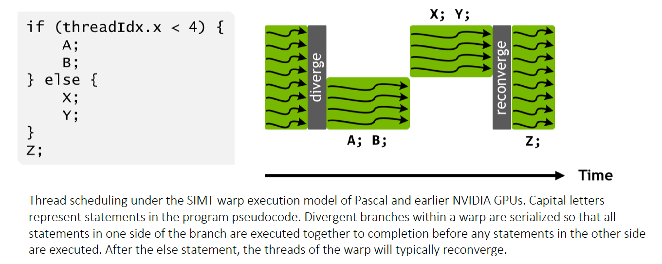
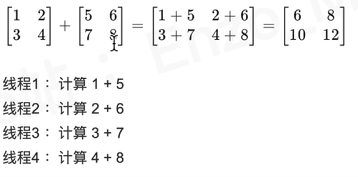
Parallel Reduction

Arithmetic intensity: compute to memory access ratio 进行一次内存访问时，可以执行多少次计算操作。这个比值越大，往往意味着性能更好。

找到数组的和，最大值，连续积，均值

Reduction:  An operation that computes a single result from a set of data

在并行计算中，为了高效地对大量数据进行规约操作（如求和、求最大值等），算法通常采用迭代的形式。在每一轮迭代中，活动的线程会将两两配对的元素进行运算，从而将数据规模减半（因为每次迭代数据都会减半，往往是$\log_2{n}$次迭代）

数组的和

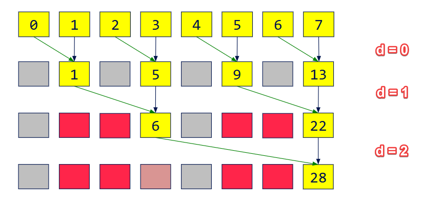
分治分冶，两个两个地求和下去
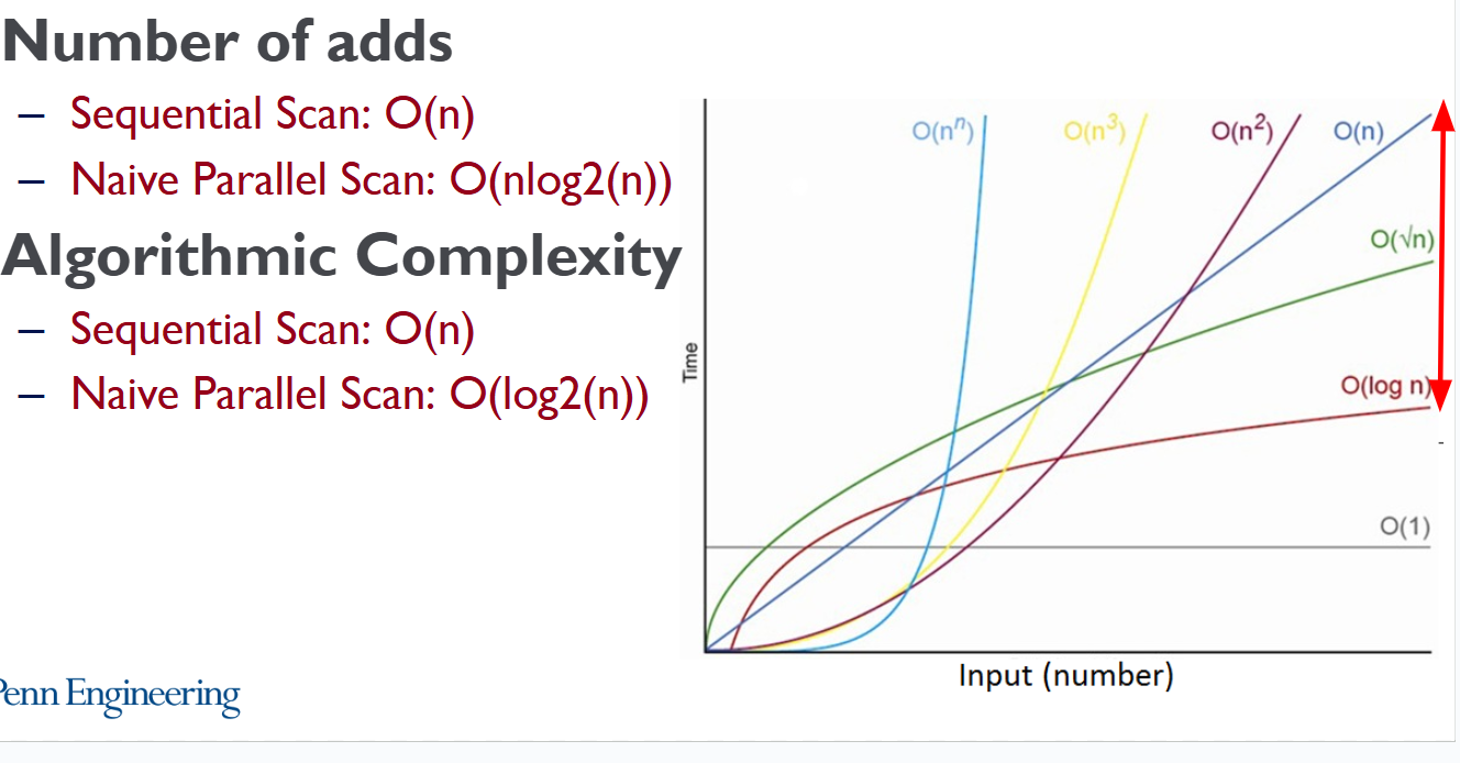
$O(logn)$ for n elements

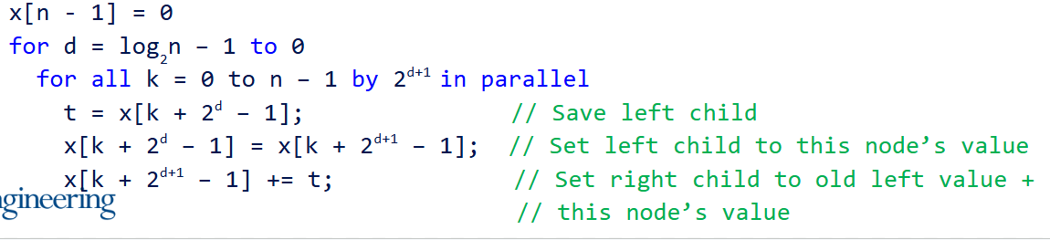
第一行的$\log_2{n} -1$ 指的是总共的迭代次数 - 1，第一行的for是用来遍历迭代的，di表示是低几次迭代

第二行的all意味着并行，k是线程的索引， 步长为$2^{d+1}$，与迭代次数有关。例如， 若若当前迭代为第0次，那么步长为$2$，如果是第1次迭代，步长为$4$，如果是第2次迭代，步长为$8$

第三行执行了加法的具体内容。

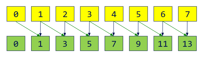
当第0次迭代时（d=0）

1
2

for all k = 0 to n -1 by 2 in parallel
	x[k + 1] += x[k]

即，
线程0，执行x[0 + 1] += x[0]，也就是 x[1] += x[0]

线程2，执行x[2 + 1] += x[2]，也就是 x[3] += x[2]

线程4，执行x[4 + 1] += x[4]，也就是 x[5] += x[4]

以此类推…

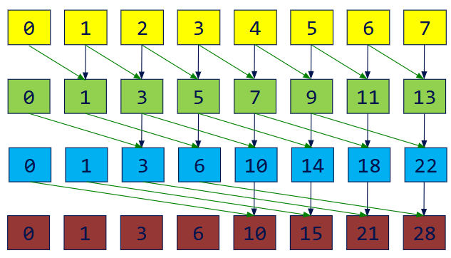
当第1次迭代时（d=1）

1
2

for all k = 0 to n -1 by 4 in parallel
	x[k + 3] += x[k + 1]

即，
线程0，执行x[0 + 3] += x[0 + 1]，也就是 x[3] += x[1]

线程4，执行x[4 + 3] += x[4 + 1]，也就是x[7] += x[5]

Scan

All-Prefix-Sums 前缀和（前缀规约）

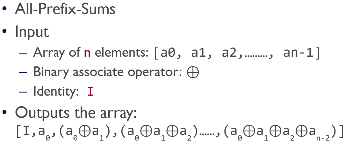
这里的⊕指的是二元运算，其需要两个操作数，且满足结合律运算，即(a⊕b)⊕c=a⊕(b⊕c)

$I$ 代表身份元，它是指与任何元素进行二元运算后，结果仍然是该元素的特殊值。

• 对于加法 (+)，身份元是 0，因为 a+0=a
• 对于乘法 (×)，身份元是 1，因为 a×1=a
• 对于最大值 (max)，身份元是 −∞ (负无穷大)，因为 max(a,−∞)=a

结合律对设计并行算法至关重要，因为它允许我们以任何顺序对数据进行分组和处理，而不会影响最终结果。

• Exclusive Scan
  不包括当前指向的数组中的元素
  In: [ 3 1 7 0 4 1 6 3]
  Out: [ 0 3 4 11 11 15 16 22]
• Inclusive Scan(Prescan) 闭扫描
  包括当前指向的数组中的元素
  In: [ 3 1 7 0 4 1 6 3]
  Out: [ 3 4 11 11 15 16 22 25]

如何从一个闭扫描创建开扫描（逆向扫描）？

Input: [ 3 4 11 11 15 16 22 25]
将每一位右移，在首位补Identity（对于这里是0），有
[ 0 3 4 11 11 15 16 22]
Exclusive: [ 0 3 4 11 11 15 16 22]

如何从一个开扫描创建闭扫描（逆向扫描） Prescan？

我们既需要开扫描，也需要原始的输入

$$
Inclusive[i]=Exclusive[i]+Input[i]
$$

将开扫描与原始输入的元素逐个相加，
得到最终结果 [ 3, 4, 11, 11, 15, 16, 22, 25]

A parallel algorithm for Inclusive Scan

对于单线程来说，这个算法很简单。首位照抄原始输入的首位，之后的元素从前一个元素加上原始输入当前的元素即可。

1
2
3

out[0] = in[0]; // assuming n > 0
for (int k = 1; k < n; ++k)
  out[k] = out[k – 1] + in[k];

若如此做，对于n个元素的数组，我们需要执行 n-1 次加法操作。

并行算法的时间复杂度是$O(logn)$，因为其不再必须等待上一步。
一般的并行化算法（Hillis-Steele）可以将工作总量变为$O(nlogn)$ ，而更高效的算法可以将工作总量优化到 $O(n)$

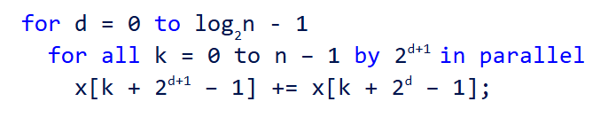
Native Parallel Scan

1
2
3
4
5

for d = 0 to (log₂n) - 1
	for all k in parallel
		if(k >= 2^(d)){
			x[k] = x[k - 2^d] + x[k];
		}

这里的d是指当前处理的是第几次迭代
注意，这里的k步长总是1， 但是其会经过$k >= 2^{d}$ 这个判断来去除一些不需要进行的运算。

由于我们无法控制线程的先后执行顺序，且算法中会出现依靠数组中其他值的情况，例如计算 Array[1] = Array[1] + Array[0]，数组中的元素可能因为被其他值更改而污染。所以在实现中使用乒乓缓存。即，在一个迭代中，只从一个数组中读，只写入另一个数组，然后交换这两个数组。

Work-Efficient Parallel Scan

若如此做，将会首先得到一个开扫描，最后进行一次逆向扫描，得到闭扫描

二叉树

利用一棵平衡二叉树来分两阶段执行Scan

假设输入是[0 1 2 3 4 5 6 7]

• Up-Sweep

1
2
3
4
5

// Same code as our Parallel Reduction
// 注意，这里的to是一个闭区间，包含log_2{n} - 1
for d = 0 to log_2{n} - 1
  for all k = 0 to n – 1 by 2^(d+1) in parallel
    x[k + 2^(d+1) – 1] += x[k + 2^(d) – 1];

% 是取模运算，a % b 的结果是 a 除以 b 后的余数。 6 % 2 = 0

需要指出的是，由于步长的存在，这里伪代码的k是一个稀疏的、跳跃式增长的变量，用来标记每个计算单元的起始位置，是从“外部调度者”的视角来看待的。而CUDA中的k，或者线程id是每个线程自己的视角，那么经过了((k + 1) % fullStride != 0) 这样的判断之后，线程id已经成为了实际写入数据的位置。

也就是说，在kernel函数中，对于每个线程而言，

1
2
3
4
5
6
7
8
9
10
11
12
13

__global__ void kernParallelScan(int paddedN, int n, int d, int* idata) {
    int k = blockIdx.x * blockDim.x + threadIdx.x;

	int halfStride = 1 << (d);
    int fullStride = halfStride * 2;

    if (k >= n || ((k + 1) % fullStride != 0)) {
        return;
    }

    // up-sweep
    idata[k] += idata[k - halfStride];
}

1. Imagine array as a tree
   Array stores only left child
   Right child is the element itself
2. For node at index n
   Left child index = n/2 (rounds down)
   Right child index = n
   

我们把这个树扫（推）上去，得到了上扫完成后的一个中间状态[0 1 2 6 4 9 6 28]

• Down-Sweep
  “下扫”的核心思想是：从树的根节点开始，将每个节点所代表的“前缀和”分配给它的子节点，直到最底层的叶子节点（也就是我们的目标数组）

1. 树顶的值换成0
2. 从上至下地，一层层地，父节点把自己的值传给左孩子，把“自己的值 + 左孩子的原始值”传给右孩子

在得到我们上扫的结果后：

我们执行下列步骤：

1. 根节点的值被设置为了0（注意，这一步应该只执行一次，而不是并行时，每个线程都这样设置一下，因为对于非第一个执行的线程，其根节点已经被第一个执行的线程更新过了）

2. 蓝色层的6，拷贝父节点的值，新值变为了0；蓝色层的22，拷贝父节点的值，加上左边兄弟的原值6，新值变为6。 也就是蓝色这一层变为了[6, 22]

3. 绿色这一层进行运算。
   绿色1，拷贝父节点的值，新值为0， 绿色5，拷贝父节点的值，加上左兄弟原值，变为1

绿色9，拷贝父节点的值6，新值为6，绿色13，拷贝父节点 6，再加上左边兄弟（绿色9）的原始值 9。新值为 6 + 9 = 15。
它们的值变成了 [0, 1, 6, 15]

5. 黄色这一层进行运算，有新的黄色层[0 0 1 3 6 10 15 21]，即开扫描

6. 将开扫描加上原始输入，有闭扫描

• Up-Sweep
  $O(n)$ adds
• Down-Sweep
  $O(n)$ adds
  $O(n)$ swaps

减少加法操作次数？

Stream Compaction

类似于std::copy_if

在GPU的时候我们就把不要的数据给丢了，这样最终需要从GPU传到CPU的
数据量就少了很多。

Why scan?

• Preserve the order
• meet certain criteria

Step 1: Compute temporary array containing

• 1 if corresponding element meets criteria
• 0 if element does not meet criteria

Step 2 Run exclusive
scan on temporary array

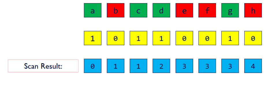
这里第一行是原始数据，绿色表示满足了条件，红色表示未满足条件

黄色是临时数组

蓝色是临时数组的开扫描

Step 3 Scatter

• Results of scan is index into final array
• Only write an element if temporary array has a 1

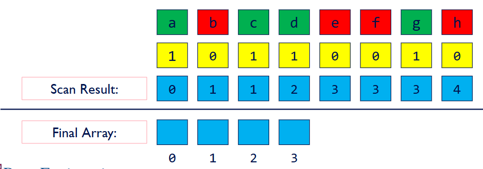
那么利用这个开扫描，我们可以知道要开一个多大的数组，也就是最后一位值，且知道每一个要写的元素将会写的index

Summed Area Table （SAT）

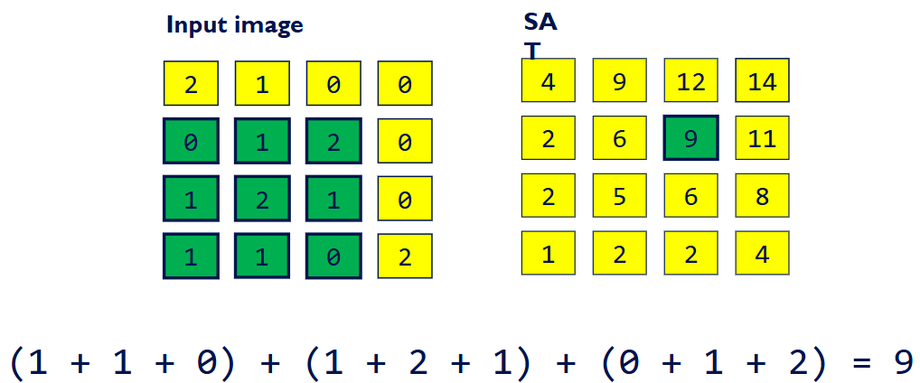
2D table where each element stores the sum of all elements in an input image between the lower left corner and the entry location.

SAT的本质是一个二维的包含式前缀和。

通过一次预计算，使得我们可以在“固定的时间”内，极速计算出图像中任意矩形区域内所有像素值的总和（以及平均值）

它的最大优点是，可以用 固定的时间O(1) 对图像的每个像素应用任意尺寸的矩形滤镜。即计算一个 3x3 小方框内所有像素的平均值，和计算一个 500x500 巨大方框内像素的平均值，花费的时间是完全相同的。

我们不需要遍历矩形内的每一个像素。我们只需要从一个预先计算好的“和区域表（SAT）”中，读取四个角点的值即可。

$$
s_{filter} = \frac{s_ur - s_ul - s_lr + s_ll}{w \times h}
$$

SAT(D) - SAT(B) - SAT(C) + SAT(A)

以近似景深为例
1.对于屏幕上的每一个像素，我们读取它的深度值。
2. 根据深度值和预设的焦距，计算出这个像素应该有多“糊”。这个模糊程度可以直接转换成一个矩形模糊窗口的尺寸（比如5x5, 15x15等）
3. 利用SAT，我们只需4次查询，就能立刻得到这个动态尺寸的矩形窗口内的像素平均值。
5. 将这个平均值作为该像素的最终颜色

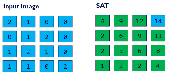
GPU Implementation Inclusive Scan

1. 原始输入

1
2
3

[ 1, 2, 3 ]
[ 4, 5, 6 ]
[ 7, 8, 9 ]

2. 水平扫描
   我们对图像的每一行，独立地执行一次包含式扫描
   第1行: [1, 1+2, 1+2+3] ➔ [ 1, 3, 6 ]

第2行: [4, 4+5, 4+5+6] ➔ [ 4, 9, 15 ]

第3行: [7, 7+8, 7+8+9] ➔ [ 7, 15, 24 ]

即

1
2
3

[ 1,  3,  6 ]
[ 4,  9, 15 ]
[ 7, 15, 24 ]

3. 垂直扫描
   我们对上一步得到的中间结果的每一列，再次独立地执行一次包含式扫描

第1列: [1, 1+4, 1+4+7] ➔ [ 1, 5, 12 ]

第2列: [3, 3+9, 3+9+15] ➔ [ 3, 12, 27 ]

第3列: [6, 6+15, 6+15+24] ➔ [ 6, 21, 45 ]

1
2
3
4

// 最终的 SAT
[  1,  3,  6 ]
[  5, 12, 21 ]
[ 12, 27, 45 ]

Radix Sort

k-bit keys require k passes k比特的键需要k轮处理

如果要对一个k比特的整数进行排序，算法需要进行k轮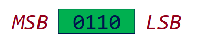

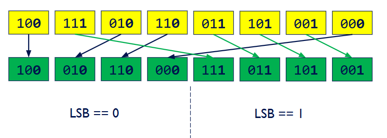
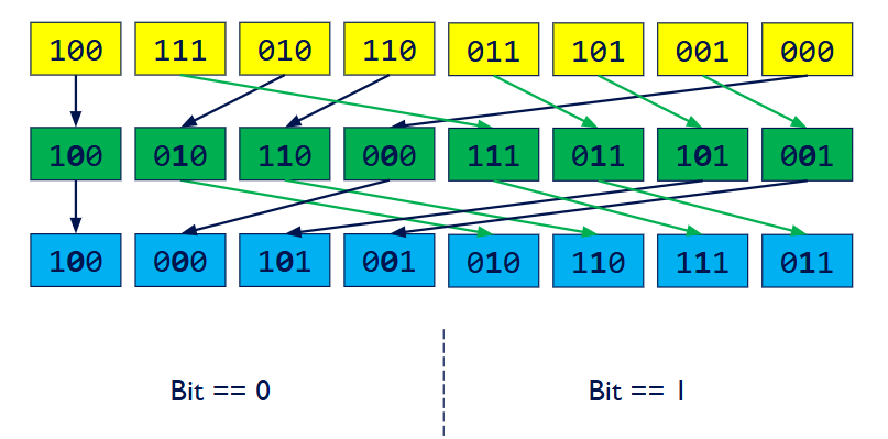
1. (Pass 1)根据所有数字的最低比特位 least significant bit (LSB)（第0位是0还是1）进行分组排序
   

2. (Pass 2)在上一轮结果的基础上，根据所有数字的次低比特位（第1位）进行分组排序
   

3. ….

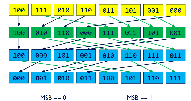
4. (Pass k)根据最高比特位most significant bit (MSB)
   

Parallel ?

1. Break input arrays into tiles

   • Each tile fits into shared memory for an SM

2. Sort tiles in parallel with radix sort

   • Each pass is done in sequence after the previous pass. No parallelism
   • Can we parallelize an individual pass? How?

3. Merge pairs of tiles using a parallel bitonic merge until all tiles are merged.

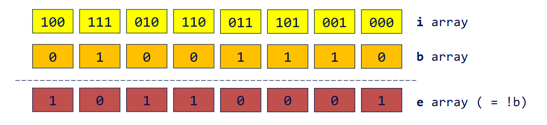
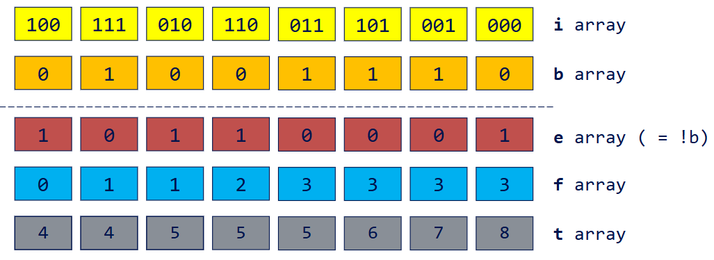
Parallel in a pass

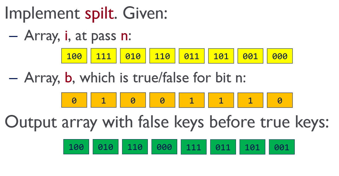
1. 计算 e 数组
   
2. 对 e 数组执行开扫描
   
3. 计算 totalFalses

1
2
3

totalFalses = e[n – 1] + f[n – 1]
totalFalses = 1 + 3
totalFalses = 4

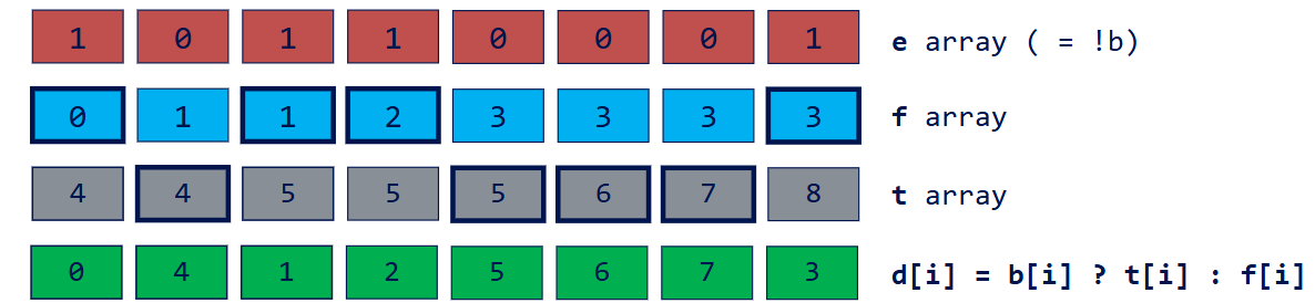
4. Compute t array

• t array is address for writing true keys

1
2

totalFalses = 4
t[i] = i – f[i] + totalFalses

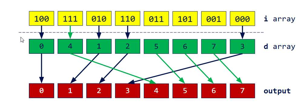
5. Scatter based on address d

1
2

d[i] = b[i] ? t[i] : f[i] 

算法将相邻的两个有序数据块（Tile 0 和 Tile 1，Tile 2 和 Tile 3，以此类推）两两配对。

GPU上的不同线程组会同时对这些数据块对执行并行的归并操作

Scan Revisited

• Limitations
  • Requires power-of-two length
  • Executes in one block (unless only using global memory)
    • Length up to twice the number of threads in a block

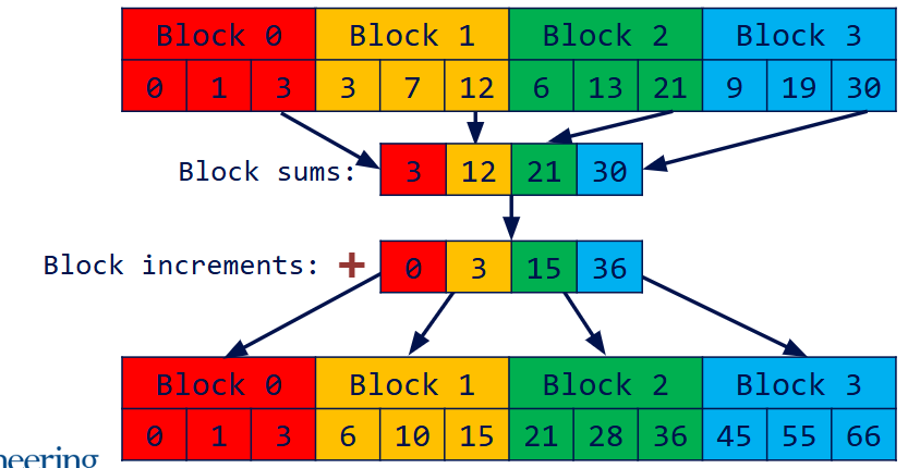
1. Devide the array into blocks
2. Run scan on each block
   
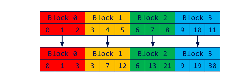
3. Write total sum of each block into a new array
   
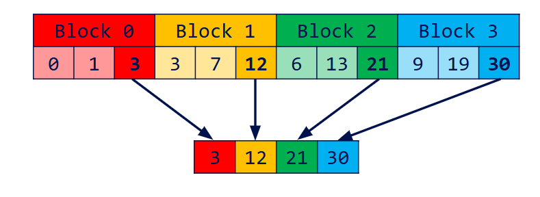
4. Exclusive scan block sums to compute block increments
   
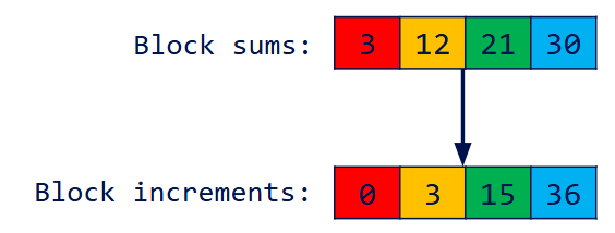
5. Add block increments to each element in the corresponding block
   

参考
2-CUDA-Introduction-2-of-2
Cuda 编程之 Tiling

Physical Architecture

NVIDIA GeForce 8800 GTX G80-300-A2

最小的单位， SP(Streaming Processor)，然后是SPs(Streaming Processors）

以 Tesla 架构的 GeForce 8 系列搭载 G80 的 8800 GTX 为例，其拥有 16 个 Streaming Multiprocessor

相比较之下，Ada LoveLace 架构的 4070 Super 其拥有56个Streaming Multiprocessor

需要注意的是，每个SM所能含有的最大threads 是随着架构的提升而增大的，不过至今的数代都保持在了2048这个数字。

Warp

Users don’t control warp, it is hardware group of 32 consecutive “lanes”(32 threads of a block)

This is why we keep threads-per-block size as multiple of 32

• Each thread occupies 1 lane, warp lanes are consecutive threadIdx values

• Unit of sheduling and execution

• CUDA GPUs schedule warps for execution, not threads

• All threads in a warp execute same instruction at the same clock-time

• Zero-overhead context switching - All resources reside on the same SM until execution

• A block will always on the same SM

• All threads in a warp execute the same insturction

  • While all threads in a grid run the same kernel code, only threads within the same warp are guaranteed to execute the same instruction at the same time.
  • They are all working from the same set of instructions, but they are not synchronized. They run independently and can be at completely different points in the program at any time.

• Swapping sheduled warps has zero overheads

• Scheduler always tries to optimize execution

• More resources required - less warp

  • Registers: A large but limited set of super-fast memory for each thread’s private variables.

  • Shared Memory: A fixed amount of fast on-chip memory allocated to thread blocks

• One SM can handle multiple block at the same time

  • Warp Size is the unit of execution.
  • Concurrent Threads is the unit of residency. This is the total number of threads that are loaded, active, and have their resources allocated on the SM, ready to be executed.

Example Ⅰ

32 threads per wap but 8 SPs per SM, What gives?

When an SM shedule its

A kernal has

• 1 global memory read
• 4 non-dependent multiples/adds

How many warps are required to hide the memory latency ?

Each warp has 4 multiples/adds
16 cycles

We need to cover 200 cycles

• 200/16 = 12.5
• ceil(12.5) = 13

13 warps are required

Example Ⅱ

• What actually happens when you launch a kernel say with 100 blocks each with 64 threads?
  • Let’s say on a GT80 (i.e. 16 SMs, 8 SPs each)
  • Max T/block is 512, Max T/SM is 768 threads
  • Chip level scheduling:
    • 100 blocks of 64 threads
    • 768/64 => max 12 blocks can be scheduled for every SM
  • SM level scheduling:
    • 12 blocks = 768 threads = 24 warps
    • Warp scheduler kicks in:
      • 8 threads -> 8 threads -> 8 threads -> 8 threads（因为这个是8 SPs each）

上述描绘了无需考虑thread所使用的resources的简化情况， 注意，每个SM这里的确可以支持12个blocks，但是100个并不是说就使用9个SM，Since your 100 blocks are fewer than the GPU’s capacity of 192, the scheduler will load all 100 blocks onto the 16 SMs immediately. Some SMs will get 6 blocks, and some will get 7, until all 100 are distributed.

Divergence

What happens if branches in a warp diverge ?

If threads within a warp take different paths in an if-else statement, the hardware has to serialize the paths, executing one after the other, which can reduce performance.

Synchronization

• Call __syncthreads();, it is on a block level

Why it is important that execution time be similar among threads ?
Long-running threads lead to inefficient stalls

Why does it only synchronize within a block?
Execution across blocks is not concurrent or ordered

Golden Role

For a __syncthreads() to work, every single thread in a block must be able to reach the same __syncthreads() call. If even one thread takes a path that skips the synchronization point, the other threads in the block will wait for it forever.

Deadlock

1
2
3
4
5
6
7
8
9
10
11
12
13
14
15
16

__global__ void faulty_kernel(float* data) {
    int idx = threadIdx.x;

    // Even and odd threads take different paths
    if (idx % 2 == 0) {
        // Even threads do some work...
        data[idx] = 1.0f;
        
        // ...and then wait here forever for the odd threads.
        __syncthreads();
    } else {
        // Odd threads are paused while the 'if' block executes.
        // They will never reach the __syncthreads() call above.
        data[idx] = 2.0f;
    }
}

1. A warp encounters an if-else statement. Some threads evaluate the condition as true, and others evaluate it as false.
2. The hardware picks one path to execute first (e.g., the if block). The threads that chose this path become active, while the threads that need to take the else path are temporarily paused (“masked off”).
3. The active threads enter the if block and hit the __syncthreads(). They now stop and wait for all other threads in their block to also arrive at this exact synchronization point.
4. Deadlock: The paused threads can never reach the __syncthreads() inside the if block because they are waiting to execute the else block. The active threads will never proceed because they are waiting for the paused threads. The entire block is now stuck in a permanent standoff.

Each __syncthreads is unique

Revisit of Matrix Multiply

The previous code:

1
2
3
4
5
6
7
8
9
10
11
12
13
14
15
16
17
18
19
20

__global__ void MatrixMultiplyKernel(const float* devM, const float* devN,
                                     float* devP, const int width)
{
int tx = threadIdx.x;
int ty = threadIdx.y;

// Initialize accumulator to 0
float pValue = 0;

// Multiply and add
for (int k = 0; k < width; k++) {
float m = devM[ty * width + k];
float n = devN[k * width + tx];
pValue += m * n;
}

// Write value to device memory - each thread has unique index to write to
devP[ty * width + tx] = pValue;
}

原来的想法很朴素，我最终的矩阵多大，我就开多少个线程去算，一个线程对应最终矩阵C的一个值。

那么这个线程去算的时候呢，要看一下矩阵A的一行，再看矩阵B的一列。最终进行乘法、相加运算。C中的每个元素的线程都要去看A和看B，那么就会带来大量的对于Global Memory的访问，这会十分低效。

直觉上打一个不恰当的比方，我们给一个大房间铺地砖的时候，应该是拿个小推车去从大货车上装个一批，然后在房间中从这个小推车上拿了地砖去铺，小推车拿空了小推车再去装一批。而不是每铺一个地砖都要去大货车中拿一块地砖。

我们要做的是，找的一种办法提升shared memory的使用，减少Global Memory的访问，这种办法可以记录某些中间状态，让矩阵C的每个元素计算不至于总是去查A和、B


图片出自Cuda 编程之 Tiling

Say, we have matrix $A$

$$
\left[ \begin{array}{cc}
2 & 6 & 7 &5 \
3 & 1 & 4 &6 \
8 & 9 & 0 &1 \
2 & 7 & 7 &4
\end{array}
\right]
$$

matrix $B$

$$
\left[ \begin{array}{cc}
1 & 6 & 2 &1 \
3 & 9 & 8 &4 \
5 & 6 & 3 &9 \
1 & 0 & 7 &2
\end{array}
\right]
$$

1
2
3
4
5
6
7
8
9
10
11
12
13
14
15
16
17
18
19
20
21
22
23
24
25
26
27
28

__global__ void MatrixMultiplyKernel(const float* devM, const float* devN,
                                     float* devP, const int width)
{
    __shared__ float sM[TILE_WIDTH][TILE_WIDTH];
    __shared__ float sN[TILE_WIDTH][TILE_WIDTH];

    int bx = blockIdx.x; 		int by = blockIdx.y;
    int tx = threadIdx.x;		int ty = threadIdx.y;

    int col = bx * width + tx;
    int row = by * width + ty;

    // Initialize accumulator to 0
    float pValue = 0;

    // Multiply and add
    for (int m = 0; m < width / TILE_WIDTH; m++) {
        sM[ty][tx] = devM[row * width + (m * TILE_WIDTH + tx)];
        sN[ty][tx] = devN[col + (m * TILE_WIDTH + ty) * Width];
        __syncthreads();

        for (int k = 0; k < TILE_WIDTH; ++k)
            pValue += sM[ty][k] * sN[k][tx];
        __syncthreads();
    }
    devP[row * width + col] = pValue;
}

for the first iteration, we have

Phase 1: Processing the First Pair of Tiles

Load Tiles into Shared Memory

matrix $sM$

$$
\left[ \begin{array}{cc}
2 & 6 \
3 & 1\
\end{array}
\right]
$$

matrix $sN$

$$
\left[ \begin{array}{cc}
1 & 6 \
3 & 9\
\end{array}
\right]
$$

__syncthreads();

Compute from Shared Memory

Our target thread (0,0) now calculates its part of the dot product using the values in the fast shared memory.

1
2
3

pValue += sM[0][0] * sN[0][0] + sM[0][1] * sN[1][0]
pValue += (2 * 1) + (6 * 3)
pValue = 20

Our target thread (0,1):

1
2
3

pValue += sM[0][0] * sN[0][1] + sM[0][1] * sN[1][1]
pValue += (2 * 6) + (6 * 9)
pValue = 66

Our target thread (1,0):

1
2
3

pValue += sM[1][0] * sN[0][0] + sM[1][1] * sN[1][0]
pValue += (3 * 1) + (1 * 3)
pValue = 6

Our target thread(1,1):

1
2
3

pValue += sM[1][0] * sN[0][1] + sM[1][1] * sN[1][1]
pValue += (3 * 6) + (1 * 9)
pValue = 27

__syncthreads();

all four of those calculations are done at the same time, in parallel.

Phase 2: Processing the Second Pair of Tiles

Load Tiles into Shared Memory

matrix $sM$

$$
\left[ \begin{array}{cc}
7 & 5 \
4 & 6\
\end{array}
\right]
$$

matrix $sN$

$$
\left[ \begin{array}{cc}
5 & 6 \
1 & 0\
\end{array}
\right]
$$

__syncthreads();

Compute from Shared Memory

Our target thread (0,0) now calculates its part of the dot product using the values in the fast shared memory.

1
2
3
4
5

pValue += sM[0][0] * sN[0][0] + sM[0][1] * sN[1][0]
pValue += (7 * 5) + (5 * 1)
pValue += 40

pValue = 60

Our target thread (0,1):

1
2
3
4
5

pValue += sM[0][0] * sN[0][1] + sM[0][1] * sN[1][1]
pValue += (7 * 6) + (5 * 0)
pValue += 42

pValue = 108

Our target thread (1,0):

1
2
3
4
5

pValue += sM[1][0] * sN[0][0] + sM[1][1] * sN[1][0]
pValue += (4 * 5) + (6 * 1)
pValue += 26

pValue = 32

Our target thread(1,1):

1
2
3
4
5

pValue += sM[1][0] * sN[0][1] + sM[1][1] * sN[1][1]
pValue += (4 * 6) + (6 * 0)
pValue += 24

pValue = 51

__syncthreads();

all four of those calculations are done at the same time, in parallel.

Now, we have the left top block of C:

$$
\left[ \begin{array}{cc}
60 & 108 \
32 & 51\
\end{array}
\right]
$$

为什么我们可以这么做？

Dot product can be done as partial nums

在naive中，我们想求一个C的元素，我们一次性去拿A的对应横行和B的对应纵行进行计算。在tiling中，我们把这个计算分为多步，对于每个我们关注的C的子矩阵，即一个block，比如例子这里就是left top block of C，我们去看原矩阵A、B对应的block，而后进行运算。这会让我们不再每求一个C的元素都要将A的对应横行和B的对应纵行全部访问一遍，而是，我关注的这个C的block在原A矩阵中的对应（横向）block 以及原B矩阵中的对应（竖向）的block块A,B,C, 做累加操作。每次我都会先缓存以下当前关注的A、B中的block，称作sM、sN
以下是block同步开始的
top left block of C

top second left block of C

CPU side serial code controls(send commands to) CPU side parallel code

• 初始化数据（在CPU内存中）
• 分配GPU内存
• 将数据从CPU内存拷贝到GPU内存
• 启动GPU上的核函数（Kernal）
• 等待GPU计算完成
• 将计算结果从GPU内存拷贝到CPU内存
• 释放GPU和CPU内存

CUDA 函数执行空间限定符

kernals are running on the GPU, so we use pointers to access memory

__global__

1

__global__ void myKernel()

• must return void
• 如果需要返回结果，必须通过传入指针，让核函数将结果写入GPU内存中
• 使用一种特殊的 <<<...>>> 执行配置语法来调用，例如 myKernal<<<grid, block>>>(args...);

__device__

1

__device__ float myDeviceFunction()

• 这是一个只能在GPU上执行，并且也只能被其他 __global__ 或 __device__ 函数调用的函数。它通常用于在核函数中实现一些可重用的辅助功能，类似于普通C++代码中的普通函数。
• Inlined by default

for all device code

• No static variables
  • lifetime of the program
  • on the gpu there is no lifetime concept
• No malloc()
  • never
  • many of threads tring to allocate, not enough cache to do that
  • compiler allows, but performance issue
  • GPU内存最好由主机端统一管理。标准的做法是在主机端使用 cudaMalloc() 分配一大块内存，然后将指向这块内存的指针传递给核函数。GPU线程在这个预先分配好的内存区域中进行读写操作。

__host__

1

__host__ int myHostFunction()

这就是一个普通的C/C++函数，在CPU上执行，也只能被CPU调用。如果不写任何限定符，函数默认就是 __host__

组合用法

__device__ __host__ void func() VALID
这意味着这个函数被编译了两次：一个版本用于在CPU上调用，另一个版本用于在GPU上调用。这在我们希望CPU和GPU共享某个工具函数（例如一个简单的数学计算）时非常有用。

__global__ __host__ void func() INVALID
这个组合在逻辑上是矛盾的。__global__ 的核心定义是“从CPU调用，在GPU执行”，而 __host__ 的定义是“从CPU调用，在CPU执行”。一个函数不能同时满足这两种执行模式，因此编译器禁止这种组合。

if __global__, it is only __global__ nothing else

pow, sqrt, exp, sin, cos
__powf, __sinf, __logf, __exp

Grid, Block, Thread

这些都是抽象的概念，并非是真是的物理结构，区分这些概念是为了更高效地编程

让不同的线程，拿不同的数据，进行相同的运算

gridDim 与 blockDim 都是dim3

上图中的, 表示1D Grid， 其在x方向上有4个Block，而其他方向上都只有1个Block （默认1个）

1

dim3 gridDim(4);

一般的，我们需要设置 block 中的每个维度的线程数为 32 的整数倍

Thread

执行计算的最基本单元。每个线程都会完整地执行一遍核函数 (__global__函数) 的代码。

Treading Model

Real world limitations
- No. of cores Cores/ Transistors for memory
- Power
- Scheduling

Thread Hierarchies

在 __global__ 函数内部，可以直接使用一些内置的只读变量来确定当前线程的位置：
dim3 gridDim 网格的维度
dim3 blockDim 线程块的维度
uint3 blockIdx 当前线程所在Block在Grid中的索引
uint3 threadIdx 当前线程在Block中的索引

1D: Thread ID == Thread Index
2D with size (Dx, Dy)
Thread ID of index (x, y) == x + y Dx
3D with size (Dx, Dy, Dz)
Thread ID of index (x, y, z) == x + y Dx + z Dx Dy

1
2
3
4
5
6
7
8
9
10
11
12
13
14
15
16
17
18
19
20
21
22
23
24
25
26
27
28
29
30
31
32
33
34
35
36
37
38
39
40
41
42
43

// Kernel function to add two matrices
__global__ void matrixAddition(const float* A, const float* B, float* C, int width, int height)
{
    // Calculate the global row and column index
    int col = blockIdx.x * blockDim.x + threadIdx.x;
    int row = blockIdx.y * blockDim.y + threadIdx.y;

    // Check if the thread is within the matrix bounds
    if (col < width && row < height) {
        int idx = row * width + col;
        C[idx] = A[idx] + B[idx];
    }
}

int main()
{
    int width = 1024;
    int height = 1024;
    int numElements = width * height;
    size_t size = numElements * sizeof(float);

    // ... (此处省略了为 A, B, C 分配主机和设备内存，以及数据拷贝的代码) ...
    // ... cudaMalloc, cudaMemcpy, etc. ...

    // Define the dimensions of the thread block
    // 通常选择一个二维的块，例如 16x16 或 32x32
    dim3 threadsPerBlock(16, 16);

    // Calculate the dimensions of the grid
    // 向上取整，确保有足够的block覆盖整个矩阵
    dim3 gridDim( (width + threadsPerBlock.x - 1) / threadsPerBlock.x,
                  (height + threadsPerBlock.y - 1) / threadsPerBlock.y );

    std::cout << "Launching Kernel with Grid: (" << gridDim.x << ", " << gridDim.y << "), Block: (" << threadsPerBlock.x << ", " << threadsPerBlock.y << ")" << std::endl;

    // Launch the kernel
    matrixAddition<<<gridDim, threadsPerBlock>>>(A_d, B_d, C_d, width, height);
    
    // ... (此处省略了将结果从C_d拷贝回C_h，以及释放内存的代码) ...
    // ... cudaMemcpy, cudaFree, free ...

    return 0;
}

Block

块内的线程可以相互协作，例如通过共享内存 (Shared Memory) 快速交换数据，也可以进行同步 (__syncthreads())。

一个块内的所有线程必须在同一个流式多处理器 (Streaming Multiprocessor, SM) 上执行

一个 Block 至多可以容纳 1024 个 Thread，这是自开普勒架构（GTX 10系列）显卡之后的规范。

但是，1024个线程并不意味着同一时间会执行1024个，最小的执行单位是Warp

1

dim3 threadsPerBlock(16, 16);

This line declares that each thread block will be a 2D grid containing 16 x 16 = 256 threads. You are creating a small, square team of threads. Here, threadsPerBlock.x is 16 and threadsPerBlock.y is 16. The z-dimension is 1 by default.

需要注意的是，这里的图片是Scalability的实例，并不是说每次SM就处理一个Block。在同一个Block上运行的threads 确实都在同一个SM上，也就意味着其都可以与L1通信，但是，通过这种办法来达成Block间的通信是不安全的。

不同块之间的线程是无法直接通信和同步的。

Grid

一组线程块的集合。
一个核函数的所有线程都组织在一个网格中