Spring - Damper

$$
f = -k_s \boldsymbol{x} - k_d \boldsymbol{v}
$$
where,
$k_s = \text{spring constant}$

$\boldsymbol{x} = \text{distance from rest state}$
$x = \vert \vert \boldsymbol{x}_1 -\boldsymbol{x}_2 \vert \vert - l$
$\hat{\boldsymbol{d}} = \frac{\boldsymbol{x}_1 - \boldsymbol{x}_2}{\vert \vert\boldsymbol{x}_1 - \boldsymbol{x}_2 \vert \vert}$
$\boldsymbol{x} = x\hat{\boldsymbol{d}}$

$k_d = \text{damping factor}$
$\boldsymbol{v} = \text{velocity along spring axis}$

Aerodynamic Forces

$f_{drag} = \frac{1}{2} \rho \vert \vert \boldsymbol{v}\vert \vert ^2 c_d A \hat{\boldsymbol{v}}$

$f_{lift} = \frac{1}{2} \rho \vert \vert \boldsymbol{v}\vert \vert ^2 c_L S(\alpha - \alpha_0)$

Simulation

General Steps

1. Compute all forces acting on each particle in the
   system in the current configuration

2. Compute the resulting acceleration for each particle
   (a=f/m)

3. Integrate over some small time step Dt to get new
   positions and velocities at next time step

4. Repeat

一般的，我们有这样的关系：
$\ddot{\boldsymbol{x}} = \frac{1}{m} \boldsymbol{f(x, \dot{x})}$ 或是，$\dot{\boldsymbol{v}} = \frac{1}{m} \boldsymbol{f(x, v)}$

可以理解为，当前的加速度由当前的位移与速度决定。例如，在一个弹簧阻尼系统中，当前受到的力是位移和速度共同决定的。

我们往往想要求一阶的表示方式$\boldsymbol{x}(t)$

Phase Space

State Position (6 x 1)
$s = \left[\begin{matrix}
\boldsymbol{x} \ \boldsymbol{v}
\end{matrix}\right]$

State Velocity (6 x 1)
$s = \left[\begin{matrix}
\dot{\boldsymbol{x}} \ \dot{\boldsymbol{v}}
\end{matrix}\right]$

Particle System Dynamics (6 x 1)

$s = \left[\begin{matrix}
\boldsymbol{v} \ \frac{\boldsymbol{f}}{m}
\end{matrix}\right]$

清空旧力 → 计算新力 → 准备数据给求解器 → 用求解器更新粒子状态

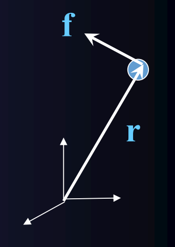
Angular Momentum: $\boldsymbol{L} = \boldsymbol{r} \times \boldsymbol{p} = \boldsymbol{r} \times m \boldsymbol{v}$

角动量可以理解为物体旋转的某种“惯性”，它是一种矢量物理量，具有大小和方向

Rate of change of Angular Momentum (力矩/扭矩)

$\boldsymbol{\tau} = \frac{d\boldsymbol{L}}{dt} = \frac{d\boldsymbol{r}}{dt} \times m\boldsymbol{v} + \boldsymbol{r} \times m \frac{d\boldsymbol{v}}{dt}$

$\boldsymbol{\tau} = \boldsymbol{r} \times \boldsymbol{f}
$
力与力臂的乘积

velocity of the particle:
$\boldsymbol{v} = \frac{d\boldsymbol{r}}{dt} = \omega \times r$

当一个刚体绕固定轴旋转时，其上的点做的是圆周运动。圆周运动的速度方向是切线方向，可以通过角速度的叉乘表达出来。

$$
\mathbf{v} = \frac{d\mathbf{r}}{dt} = \dot{\mathbf{r}} = \boldsymbol{\omega} \times \mathbf{r}
$$

Acceleration:

$$
\mathbf{a} = \frac{d\mathbf{v}}{dt} = \frac{d\boldsymbol{\omega}}{dt} \times \mathbf{r} + \boldsymbol{\omega} \times \frac{d\mathbf{r}}{dt}
$$

$$
\quad = \dot{\boldsymbol{\omega}} \times \mathbf{r} + \boldsymbol{\omega} \times (\boldsymbol{\omega} \times \mathbf{r})
$$

当角加速度为零时：
$$\dot{\boldsymbol{\omega}} = 0 $$

• Centripetal acceleration
  $$
  \mathbf{a} = \boldsymbol{\omega} \times (\boldsymbol{\omega} \times \mathbf{r})
  $$

• Centrifugal force
  $$
  \mathbf{f}_{\text{centrifugal}} = -m \boldsymbol{\omega} \times (\boldsymbol{\omega} \times \mathbf{r})
  $$

If the length of $\mathbf{r}$ is changing as a function of time then,
Velocity:

$$
\mathbf{v} = \frac{d\mathbf{r}}{dt} = \boldsymbol{\omega} \times \mathbf{r} + \mathbf{v}_r
$$

Acceleration:

$$
\frac{d\mathbf{v}}{dt} = \frac{d\boldsymbol{\omega}}{dt} \times \mathbf{r}

• \boldsymbol{\omega} \times \frac{d\mathbf{r}}{dt}
• \frac{d\mathbf{v}_r}{dt}
  $$

$$
= \dot{\boldsymbol{\omega}} \times \mathbf{r}

• \boldsymbol{\omega} \times \dot{\mathbf{r}}
• \dot{\mathbf{v}}_r
  $$

因为：

$$
\dot{\mathbf{r}} = \boldsymbol{\omega} \times \mathbf{r} + \mathbf{v}_r
$$

所以：

$$
\mathbf{a} = \dot{\boldsymbol{\omega}} \times \mathbf{r}

• \boldsymbol{\omega} \times (\boldsymbol{\omega} \times \mathbf{r})
• \dot{\mathbf{v}}_r
  $$

Rewriting Angular Momentum
$$
\mathbf{L} = \mathbf{r} \times \mathbf{p} = \mathbf{r} \times (m\mathbf{v}) = m\mathbf{r} \times \mathbf{v}
= m\mathbf{r} \times (\boldsymbol{\omega} \times \mathbf{r}) = -m \mathbf{r} \times \mathbf{r} \times \boldsymbol{\omega}
$$

这里的 𝑟 表示的是：

质点（或物体上某一点）相对于旋转轴/参考点的位置向量。

🔹 Replace $\mathbf{r} \times$ with a cross product equivalent matrix $\boldsymbol{\Gamma}$ , where:
$$
\boldsymbol{\Gamma} =
\begin{bmatrix}
0 & -r_z & r_y \
r_z & 0 & -r_x \
-r_y & r_x & 0
\end{bmatrix}
$$

🔹 This allows:
$$
\mathbf{L} = -m \mathbf{r} \times (\mathbf{r} \times \boldsymbol{\omega}) = -m \boldsymbol{\Gamma} \cdot \boldsymbol{\Gamma} \cdot \boldsymbol{\omega}
$$

🔹 Define Moment of Inertia Matrix:
$$
\mathbf{I} = -m \boldsymbol{\Gamma} \cdot \boldsymbol{\Gamma}
$$

🔹 Results in the Angular Momentum equation:
$$
\mathbf{L} = \mathbf{I} \cdot \boldsymbol{\omega}
$$

Integration

当我们知道一个关系后，例如first-order ODE form：

$\dot{\boldsymbol{x}} = \boldsymbol{f(x,u)}$ ，我们想知道 $\boldsymbol{x}(t)$

根据泰勒展开公式，有
$$\mathbf{x}(t_0 + \Delta t) =
\mathbf{x}(t_0) +
\frac{d\mathbf{x}}{dt}(t_0) \Delta t +
\frac{1}{2!} \frac{d^2 \mathbf{x}}{dt^2}(t_0) \Delta t^2 +
\frac{1}{3!} \frac{d^3 \mathbf{x}}{dt^3}(t_0) \Delta t^3 + \cdots$$

换一种写法：用离散帧时间 $t_k$

可以把时间离散成一帧一帧（每一帧时长为 $\Delta t$）：

$$\mathbf{x}(t_{k+1}) \approx \mathbf{x}(t_k) +
\dot{\mathbf{x}}(t_k)\Delta t +
\frac{1}{2!} \ddot{\mathbf{x}}(t_k)\Delta t^2 +
\frac{1}{3!} \dot{\ddot{\mathbf{x}}}(t_k)\Delta t^3 + \cdots$$

高次的项可以由链式法则求得

仅保留一阶的项时，有
$$\mathbf{x}(t_{k+1}) \approx \mathbf{x}(t_k) +
\dot{\mathbf{x}}(t_k)\Delta t $$
此处，
$$
\dot{\mathbf{x}}(t_k) = \mathbf{f(x(t_k), u(t_k) )}
$$

这样做的话如果时间间隔过长，会很不稳定。

我们考虑使用 $2^{nd} \text{Order Runge Kutta}$
Step 1.
使用欧拉方法计算 预测值
$
\mathbf{x}^p(t_{k+1}) = \mathbf{x}(t_k) + \dot{\mathbf{x}}(t_k)\Delta t
$
而后，讲此预测值带入到关系中，有

$
\dot{\mathbf{x}}^p(t_{k+1}) = f(\mathbf{x}^p(t_{k+1}), \mathbf{u}(t_k))
$

最后求取一个平均值
$
\mathbf{x}(t_{k+1}) = \mathbf{x}(t_k) + \frac{\Delta t}{2} \left[
\dot{\mathbf{x}}(t_k) + \dot{\mathbf{x}}^p(t_{k+1})
\right]
$

4ᵗʰ Order Runge Kutta

$
\mathbf{x}(t_{k+1}) = \mathbf{x}(t_k) + \frac{1}{6} \left[ \mathbf{d}_1 + 2\mathbf{d}_2 + 2\mathbf{d}_3 + \mathbf{d}_4 \right]
$

---

🔹 Where:

$
\mathbf{d}_1 = \Delta t \cdot \dot{\mathbf{x}}(t_k) = \Delta t \cdot \mathbf{f}(\mathbf{x}(t_k), \mathbf{u}(t_k))
$

$
\mathbf{d}_2 = \Delta t \cdot \mathbf{f} \left(t_k + \frac{\Delta t}{2}, \mathbf{x}(t_k) + \frac{1}{2}\mathbf{d}_1 \right)
$

$
\mathbf{d}_3 = \Delta t \cdot \mathbf{f} \left(t_k + \frac{\Delta t}{2}, \mathbf{x}(t_k) + \frac{1}{2}\mathbf{d}_2 \right)
$

$
\mathbf{d}_4 = \Delta t \cdot \mathbf{f} \left(t_k + \Delta t, \mathbf{x}(t_k) + \mathbf{d}_3 \right)
$

🔁 Backwards Euler:

$
\mathbf{x}(t_k) = \mathbf{x}(t_{k+1}) - \dot{\mathbf{x}}(t_{k+1}) \Delta t
$

or equivalently:

$
\mathbf{x}(t_{k+1}) = \mathbf{x}(t_k) + \dot{\mathbf{x}}(t_{k+1}) \Delta t
$

问题是，我们怎么算 $\dot{\mathbf{x}}(t_{k+1})$

①根据我们已知的关系，
我们${\boldsymbol{\dot {x}}(t_{k+1})} = \boldsymbol{f}(\boldsymbol{x}(t_{k+1}))$
但是我们不知道$\boldsymbol{x}(t_{k+1})$， 我们使用RK2来估算这个值

②一般的，我们使用泰勒展开
$$
\boldsymbol{x}(t_{k+1}) = \boldsymbol x(t_k) + \Delta t \cdot \dot{ \boldsymbol{x}}(t_{k+1}) \ = \boldsymbol{x}(t_{k}) + \Delta \boldsymbol{x}(t_k)
$$
$\dot{\mathbf{x}}(t_{k+1}) = \boldsymbol{f}(\boldsymbol{x}(t_{k+1})) = \boldsymbol{f}(\boldsymbol{x}(t_{k}) + \Delta \boldsymbol{x}(t_k))$

$\boldsymbol{x}(t_{k}) + \Delta \boldsymbol{x}(t_k) = \boldsymbol{x}(t_k) + \Delta t \cdot \boldsymbol{f}(\boldsymbol{x}(t_{k}) + \Delta \boldsymbol{x}(t_k))$

$
\mathbf{x}(t_{k+1}) = \mathbf{x}(t_k) + \Delta \mathbf{x}(t_k)
$

$
\mathbf{x}(t_{k+1}) = \mathbf{x}(t_k) +
\left( \frac{1}{\Delta t} \mathbf{I} - \frac{\partial \mathbf{f}}{\partial \mathbf{x}} (t_k) \right)^{-1}
\mathbf{f}(\mathbf{x}(t_k))
$

设：

$$\mathbf{f}(x, y) =
\begin{bmatrix}
f_1(x, y) = x^2 + y \
f_2(x, y) = \sin(xy)
\end{bmatrix}$$

则 Jacobian 是：

$$\frac{\partial \mathbf{f}}{\partial \mathbf{x}} =
\begin{bmatrix}
\frac{\partial f_1}{\partial x} & \frac{\partial f_1}{\partial y} \
\frac{\partial f_2}{\partial x} & \frac{\partial f_2}{\partial y}
\end{bmatrix}

\begin{bmatrix}
2x & 1 \
y\cos(xy) & x\cos(xy)
\end{bmatrix}$$

Adams Bashforth

🔹 Keep terms up to 2ⁿᵈ order in Taylor series approx

$$
\mathbf{x}(t_{k+1}) = \mathbf{x}(t_k) + \dot{\mathbf{x}}(t_k),\Delta t

• \frac{1}{2!},\ddot{\mathbf{x}}(t_k),\Delta t^2
  $$

---

🔹 Approximate the second derivative as

$$
\ddot{\mathbf{x}}(t_k)
\approx
\frac{\dot{\mathbf{x}}(t_k) - \dot{\mathbf{x}}(t_{k-1})}{\Delta t}
$$

---

🔹 Which yields

$$
\mathbf{x}(t_{k+1})
= \mathbf{x}(t_k)

• \frac{\Delta t}{2},\bigl[3,\dot{\mathbf{x}}(t_k) - \dot{\mathbf{x}}(t_{k-1})\bigr]
  $$

Verlet Integration

🔹 Does not require velocity to be explicitly computed

---

🔹 Given the current value of $\mathbf{x}(t_k)$, compute $\mathbf{x}$ at the next time step $t_{k+1}$ and previous time step $t_{k-1}$using a 2ⁿᵈ order approximation:

$$
\mathbf{x}(t_{k+1}) = \mathbf{x}(t_k) + \dot{\mathbf{x}}(t_k) \Delta t + \frac{1}{2} \ddot{\mathbf{x}}(t_k) \Delta t^2
$$

$$
\mathbf{x}(t_{k-1}) = \mathbf{x}(t_k) - \dot{\mathbf{x}}(t_k) \Delta t + \frac{1}{2} \ddot{\mathbf{x}}(t_k) \Delta t^2
$$

---

🔹 Adding the two together and rearranging yields:

$$
\mathbf{x}(t_{k+1}) = 2\mathbf{x}(t_k) - \mathbf{x}(t_{k-1}) + \ddot{\mathbf{x}}(t_k) \Delta t^2
$$

Deformation map and deformation gradient

${\pmb{R}^3 = }$ all vectors with 3 real components.

${\pmb{R}^n = }$ all vectors with n real components.

When the object undergoes deformation, every material point $\vec{X}$ is being displaced to a new deformed location which is, by convention, denoted by a lowercase variable $\vec{x}$ The relation between each material point and its deformation function $\vec{\phi} : R^{3} \rightarrow R^{3} $.
$$
\vec{x} = \vec{\phi}(\vec{X})·1
$$
An important physical quantity derived directly from $\vec{\phi}(\vec{X})$, is the deformation gradient tensor ${ \pmb{F} \in \pmb{R^{3\times3}}}$

If we write ${\vec{X} = (X_1,X_2,X_3)^T} or{\vec{X} = (X,Y,Z)^T} $ and ${\vec{\phi}(\vec{X}) = (\vec{\phi_1}(\vec{X}),\vec{\phi_2}(\vec{X}),\vec{\phi_3}(\vec{X}))^T}$

注意是原每一组点根据三个对应关系被分别转换到三个分量上

for the three components of the vector-valued function ${\vec{\phi}}$, the deformation gradient is written as:
$$
\pmb{F}:= \frac{\partial(\phi_1,\phi_2,\phi_3)}{\partial({X_1,X_2,X_3})} = \left( \begin{matrix}\frac{\partial\phi_1}{\partial X_1} & \frac{\partial\phi_1}{\partial X_2} & \frac{\partial\phi_1}{\partial X_3}\
\frac{\partial\phi_2}{\partial X_1} & \frac{\partial\phi_2}{\partial X_2} & \frac{\partial\phi_2}{\partial X_3}\
\frac{\partial\phi_3}{\partial X_1} & \frac{\partial\phi_3}{\partial X_2} & \frac{\partial\phi_3}{\partial X_3}\end{matrix}\right)
$$
or, in index notation ${ F_{ij} = \phi_{i,j} }$ . In simple terms, the deformation gradient measures the amount of change in shape and size of a material body relative to its original configuration. The magnitude of the deformation gradient can be used to determine the amount of deformation or strain that has occurred, and its orientation can be used to determine the direction of deformation.

Note that, in general, $\pmb{F}$ will be spatially varying across ${\Omega}$, which is the volumetric domain occupied by the object. This domain will be referred to as the reference(or undefined configuration)

Strain energy and hyperelasticity

One of the consequences of elastic deformation is the accumulation of potential energy in the deformed body, which is referred to as strain energy ${E[\phi]}$ in the context of deformable solids. It is suggested that the energy is fully determined by the deformation map of a given configuration.

However intuitive, this statement nevertheless reflects a significant hypothesis that led to this formulation: we have assumed that the potential energy associated with a deformed configuration only depends on the final deformed shape, and not on the deformation path over time that brought the body into its current configuration.

The independence of the strain energy on the prior deformation history is a characteristic property of so-called hyperelastic materials. This property of is closely related with the fact that elastic forces of hyperelastic materials are conservative: the total work done by the internal elastic forces in a deformation path depends solely on the initial and final configurations, not the path itself.

Different parts of a deforming body undergo shape changes of different severity. As a consequence, the relation between deformation and strain energy is better defined on a local scale. We achieve that by introducing an energy density function ${\Psi[\phi;\vec{X}]}$ which measures the strain energy per unit undeformed volume on an infinitesimal domain ${dV}$ around the material point $\vec{X}$. We can then obtain the total energy for the deforming body by integrating the energy density function over the entire domain ${\Omega}$:
$$
E[\phi] = \int_\Omega\Psi[\phi;\vec{X}]d\vec{X}
$$